This lab is due on Monday, September 22 at 11:59pm. To be considered on time, the following must be done by the due date:
Final .pdf file submitted on Gradescope
Introduction
The main goal is to learn data processsing using tidyverse and introduce you to version control using Github. Most of these labs is adopted from Nick Hagerty course materials.
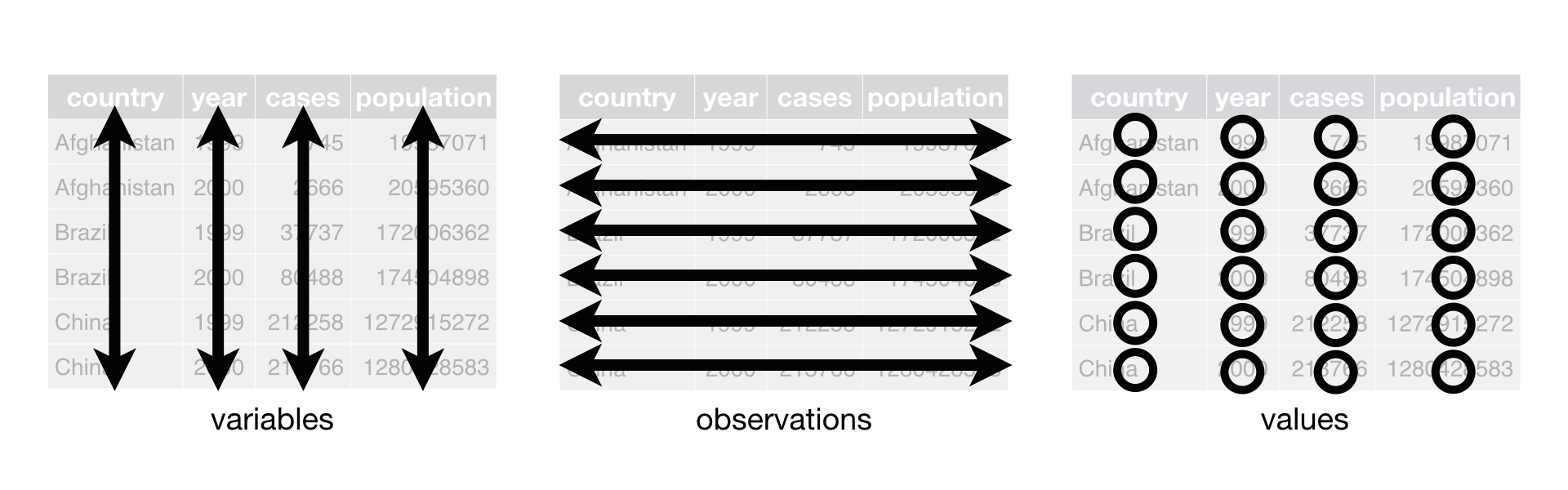
Tidy data is easier to work with, because you have a consistent way of referring to variables and observations. It then becomes easy to manipulate, visualize, and model.
Wide vs. Long Formats
Both of these data sets display information on heart rate observed in individuals across 3 different time periods:
Row = patient. Columns = repeated observations over time.
Often easier to take in at a glance (as in a spreadsheet).
Long data:
Row = one observation. Columns = ID variables + observed variable.
Usually easier to clean, merge with other data, and avoid errors.
Tidy data is more likely to be long.
Most R packages have been written assuming your data is in long format.
“Tidy datasets are all alike but every messy dataset is messy in its own way.”
– Hadley Wickham
Tidyverse packages
We need to install and load a couple of packages. Run these preliminaries:
# load and install package if necessaryif (!require("pacman")) install.packages("pacman")pacman::p_load( tidyverse, nycflights13 )
We see that we have actually loaded a number of packages (which could also be loaded individually): ggplot2, tibble, dplyr, etc. - We can also see information about the package versions and some namespace conflicts.
The tidyverse actually comes with a lot more packages than those that are just loaded automatically.
# A tibble: 3 × 2
  model      hwy_mean
  <chr>         <dbl>
1 a4             28.3
2 a4 quattro     25.8
3 a6 quattro     24
Vertical space costs nothing and makes for much more readable/writable code than cramming things horizontally.
All together, this multi-line line of code is called a pipeline.
Key dplyr verbs
There are five key dplyr verbs that you need to learn.
filter: Filter (i.e. subset) rows based on their values.
arrange: Arrange (i.e. reorder) rows based on their values.
select: Select (i.e. subset) columns by their names:
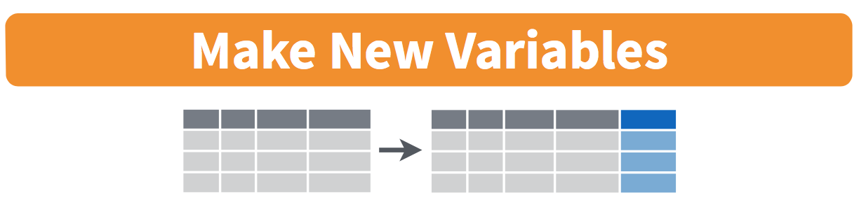
mutate: Create new columns.
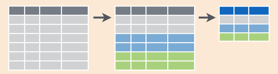
summarize: Collapse multiple rows into a single summary value.
Let’s practice these functions together using the starwars data frame that comes pre-packaged with dplyr.
Exercise 1: dplyr::filter
We can chain multiple filter commands with the pipe (|>), or just separate them within a single filter command using commas.
starwars |>filter( species =="Human", height >=190 )
# A tibble: 4 × 14
  name      height  mass hair_color skin_color eye_color birth_year sex   gender
  <chr>      <int> <dbl> <chr>      <chr>      <chr>          <dbl> <chr> <chr>
1 Darth Va…    202   136 none       white      yellow          41.9 male  mascu…
2 Qui-Gon …    193    89 brown      fair       blue            92   male  mascu…
3 Dooku        193    80 white      fair       brown          102   male  mascu…
4 Bail Pre…    191    NA black      tan        brown           67   male  mascu…
# ℹ 5 more variables: homeworld <chr>, species <chr>, films <list>,
#   vehicles <list>, starships <list>
Regular expressions work well too.
starwars |>filter(str_detect(name, "Skywalker"))
# A tibble: 3 × 14
  name      height  mass hair_color skin_color eye_color birth_year sex   gender
  <chr>      <int> <dbl> <chr>      <chr>      <chr>          <dbl> <chr> <chr>
1 Luke Sky…    172    77 blond      fair       blue            19   male  mascu…
2 Anakin S…    188    84 blond      fair       blue            41.9 male  mascu…
3 Shmi Sky…    163    NA black      fair       brown           72   fema… femin…
# ℹ 5 more variables: homeworld <chr>, species <chr>, films <list>,
#   vehicles <list>, starships <list>
A very common filter use case is identifying (or removing) missing data cases.
starwars |>filter(is.na(height))
# A tibble: 6 × 14
  name      height  mass hair_color skin_color eye_color birth_year sex   gender
  <chr>      <int> <dbl> <chr>      <chr>      <chr>          <dbl> <chr> <chr>
1 Arvel Cr…     NA    NA brown      fair       brown             NA male  mascu…
2 Finn          NA    NA black      dark       dark              NA male  mascu…
3 Rey           NA    NA brown      light      hazel             NA fema… femin…
4 Poe Dame…     NA    NA brown      light      brown             NA male  mascu…
5 BB8           NA    NA none       none       black             NA none  mascu…
6 Captain …     NA    NA none       none       unknown           NA fema… femin…
# ℹ 5 more variables: homeworld <chr>, species <chr>, films <list>,
#   vehicles <list>, starships <list>
To remove missing observations, simply use negation: filter(!is.na(height)).
Try this yourself.
# A tibble: 6 × 14
  name      height  mass hair_color skin_color eye_color birth_year sex   gender
  <chr>      <int> <dbl> <chr>      <chr>      <chr>          <dbl> <chr> <chr>
1 Arvel Cr…     NA    NA brown      fair       brown             NA male  mascu…
2 Finn          NA    NA black      dark       dark              NA male  mascu…
3 Rey           NA    NA brown      light      hazel             NA fema… femin…
4 Poe Dame…     NA    NA brown      light      brown             NA male  mascu…
5 BB8           NA    NA none       none       black             NA none  mascu…
6 Captain …     NA    NA none       none       unknown           NA fema… femin…
# ℹ 5 more variables: homeworld <chr>, species <chr>, films <list>,
#   vehicles <list>, starships <list>
Exercise 2: dplyr::arrange
arrange sorts your data frame by a particular column (numerically, or alphabetically)
starwars |>arrange(birth_year)
# A tibble: 87 × 14
   name     height  mass hair_color skin_color eye_color birth_year sex   gender
   <chr>     <int> <dbl> <chr>      <chr>      <chr>          <dbl> <chr> <chr>
 1 Wicket …     88  20   brown      brown      brown            8   male  mascu…
 2 IG-88       200 140   none       metal      red             15   none  mascu…
 3 Luke Sk…    172  77   blond      fair       blue            19   male  mascu…
 4 Leia Or…    150  49   brown      light      brown           19   fema… femin…
 5 Wedge A…    170  77   brown      fair       hazel           21   male  mascu…
 6 Plo Koon    188  80   none       orange     black           22   male  mascu…
 7 Biggs D…    183  84   black      light      brown           24   male  mascu…
 8 Han Solo    180  80   brown      fair       brown           29   male  mascu…
 9 Lando C…    177  79   black      dark       brown           31   male  mascu…
10 Boba Fe…    183  78.2 black      fair       brown           31.5 male  mascu…
# ℹ 77 more rows
# ℹ 5 more variables: homeworld <chr>, species <chr>, films <list>,
#   vehicles <list>, starships <list>
We can also arrange items in descending order using arrange(desc()).
starwars |>arrange(desc(birth_year))
# A tibble: 87 × 14
   name     height  mass hair_color skin_color eye_color birth_year sex   gender
   <chr>     <int> <dbl> <chr>      <chr>      <chr>          <dbl> <chr> <chr>
 1 Yoda         66    17 white      green      brown            896 male  mascu…
 2 Jabba D…    175  1358 <NA>       green-tan… orange           600 herm… mascu…
 3 Chewbac…    228   112 brown      unknown    blue             200 male  mascu…
 4 C-3PO       167    75 <NA>       gold       yellow           112 none  mascu…
 5 Dooku       193    80 white      fair       brown            102 male  mascu…
 6 Qui-Gon…    193    89 brown      fair       blue              92 male  mascu…
 7 Ki-Adi-…    198    82 white      pale       yellow            92 male  mascu…
 8 Finis V…    170    NA blond      fair       blue              91 male  mascu…
 9 Palpati…    170    75 grey       pale       yellow            82 male  mascu…
10 Cliegg …    183    NA brown      fair       blue              82 male  mascu…
# ℹ 77 more rows
# ℹ 5 more variables: homeworld <chr>, species <chr>, films <list>,
#   vehicles <list>, starships <list>
Exercise 3: dplyr::select
Use commas to select multiple columns out of a data frame. (You can also use “first:last” for consecutive columns). Deselect a column with “-”.
# A tibble: 87 × 5
   name                mass hair_color    skin_color  species
   <chr>              <dbl> <chr>         <chr>       <chr>
 1 Luke Skywalker        77 blond         fair        Human
 2 C-3PO                 75 <NA>          gold        Droid
 3 R2-D2                 32 <NA>          white, blue Droid
 4 Darth Vader          136 none          white       Human
 5 Leia Organa           49 brown         light       Human
 6 Owen Lars            120 brown, grey   light       Human
 7 Beru Whitesun Lars    75 brown         light       Human
 8 R5-D4                 32 <NA>          white, red  Droid
 9 Biggs Darklighter     84 black         light       Human
10 Obi-Wan Kenobi        77 auburn, white fair        Human
# ℹ 77 more rows
You can also rename some (or all) of your selected variables in place.
starwars |>select(alias=name, planet=homeworld)
# A tibble: 87 × 2
   alias              planet
   <chr>              <chr>
 1 Luke Skywalker     Tatooine
 2 C-3PO              Tatooine
 3 R2-D2              Naboo
 4 Darth Vader        Tatooine
 5 Leia Organa        Alderaan
 6 Owen Lars          Tatooine
 7 Beru Whitesun Lars Tatooine
 8 R5-D4              Tatooine
 9 Biggs Darklighter  Tatooine
10 Obi-Wan Kenobi     Stewjon
# ℹ 77 more rows
If you just want to rename columns without subsetting them, you can use rename. Try this!
The select(contains(PATTERN)) option provides a nice shortcut in relevant cases.
starwars |>select(name, contains("color"))
# A tibble: 87 × 4
   name               hair_color    skin_color  eye_color
   <chr>              <chr>         <chr>       <chr>
 1 Luke Skywalker     blond         fair        blue
 2 C-3PO              <NA>          gold        yellow
 3 R2-D2              <NA>          white, blue red
 4 Darth Vader        none          white       yellow
 5 Leia Organa        brown         light       brown
 6 Owen Lars          brown, grey   light       blue
 7 Beru Whitesun Lars brown         light       blue
 8 R5-D4              <NA>          white, red  red
 9 Biggs Darklighter  black         light       brown
10 Obi-Wan Kenobi     auburn, white fair        blue-gray
# ℹ 77 more rows
Some other selection helpers: starts_with(), ends_with(), all_of(c("name1", "name2")), matches().
Exercise 4: dplyr::mutate
You can create new columns from scratch, or (more commonly) as transformations of existing columns.
starwars |>select(name, birth_year) |>mutate(dog_years = birth_year *7) |>mutate(comment =paste0(name, " is ", dog_years, " in dog years."))
# A tibble: 87 × 4
   name               birth_year dog_years comment
   <chr>                   <dbl>     <dbl> <chr>
 1 Luke Skywalker           19        133  Luke Skywalker is 133 in dog years.
 2 C-3PO                   112        784  C-3PO is 784 in dog years.
 3 R2-D2                    33        231  R2-D2 is 231 in dog years.
 4 Darth Vader              41.9      293. Darth Vader is 293.3 in dog years.
 5 Leia Organa              19        133  Leia Organa is 133 in dog years.
 6 Owen Lars                52        364  Owen Lars is 364 in dog years.
 7 Beru Whitesun Lars       47        329  Beru Whitesun Lars is 329 in dog yea…
 8 R5-D4                    NA         NA  R5-D4 is NA in dog years.
 9 Biggs Darklighter        24        168  Biggs Darklighter is 168 in dog year…
10 Obi-Wan Kenobi           57        399  Obi-Wan Kenobi is 399 in dog years.
# ℹ 77 more rows
Note:mutate is order aware. So you can chain multiple mutates in a single call.
starwars |>select(name, birth_year) |>mutate(dog_years = birth_year *7, # Separate with a commacomment =paste0(name, " is ", dog_years, " in dog years.") )
# A tibble: 87 × 4
   name               birth_year dog_years comment
   <chr>                   <dbl>     <dbl> <chr>
 1 Luke Skywalker           19        133  Luke Skywalker is 133 in dog years.
 2 C-3PO                   112        784  C-3PO is 784 in dog years.
 3 R2-D2                    33        231  R2-D2 is 231 in dog years.
 4 Darth Vader              41.9      293. Darth Vader is 293.3 in dog years.
 5 Leia Organa              19        133  Leia Organa is 133 in dog years.
 6 Owen Lars                52        364  Owen Lars is 364 in dog years.
 7 Beru Whitesun Lars       47        329  Beru Whitesun Lars is 329 in dog yea…
 8 R5-D4                    NA         NA  R5-D4 is NA in dog years.
 9 Biggs Darklighter        24        168  Biggs Darklighter is 168 in dog year…
10 Obi-Wan Kenobi           57        399  Obi-Wan Kenobi is 399 in dog years.
# ℹ 77 more rows
Boolean, logical and conditional operators all work well with mutate too.
# A tibble: 87 × 6
   name               height  mass hair_color    skin_color  eye_color
   <chr>               <int> <dbl> <chr>         <chr>       <chr>
 1 LUKE SKYWALKER        172    77 BLOND         FAIR        BLUE
 2 C-3PO                 167    75 <NA>          GOLD        YELLOW
 3 R2-D2                  96    32 <NA>          WHITE, BLUE RED
 4 DARTH VADER           202   136 NONE          WHITE       YELLOW
 5 LEIA ORGANA           150    49 BROWN         LIGHT       BROWN
 6 OWEN LARS             178   120 BROWN, GREY   LIGHT       BLUE
 7 BERU WHITESUN LARS    165    75 BROWN         LIGHT       BLUE
 8 R5-D4                  97    32 <NA>          WHITE, RED  RED
 9 BIGGS DARKLIGHTER     183    84 BLACK         LIGHT       BROWN
10 OBI-WAN KENOBI        182    77 AUBURN, WHITE FAIR        BLUE-GRAY
# ℹ 77 more rows
Exercise 5: dplyr::summarize
Particularly useful in combination with the group_by command.
# A tibble: 38 × 4
   species   height  mass birth_year
   <chr>      <dbl> <dbl>      <dbl>
 1 Aleena       79     15         NA
 2 Besalisk    198    102         NA
 3 Cerean      198     82         92
 4 Chagrian    196     NA         NA
 5 Clawdite    168     55         NA
 6 Droid        NA     NA         NA
 7 Dug         112     40         NA
 8 Ewok         88     20          8
 9 Geonosian   183     80         NA
10 Gungan      209.    NA         NA
# ℹ 28 more rows
The same across-based workflow that we saw with mutate a few slides back also works with summarize. Though to add arguments, we have to use an anonymous function:
# A tibble: 38 × 4
   species   height  mass birth_year
   <chr>      <dbl> <dbl>      <dbl>
 1 Aleena       79   15        NaN
 2 Besalisk    198  102        NaN
 3 Cerean      198   82         92
 4 Chagrian    196  NaN        NaN
 5 Clawdite    168   55        NaN
 6 Droid       131.  69.8       53.3
 7 Dug         112   40        NaN
 8 Ewok         88   20          8
 9 Geonosian   183   80        NaN
10 Gungan      209.  74         52
# ℹ 28 more rows
Other dplyr goodies
ungroup: For ungrouping after using group_by. - Use after doing your grouped summarize or mutate operation, or everything else you do will be super slow.
slice: Subset rows by position rather than filtering by values. - E.g. starwars |> slice(1:10)
pull: Extract a column from as a data frame as a vector or scalar. - E.g. starwars |> filter(sex=="female") |> pull(height)
distinct and count: List unique values, with or without their number of appearances. - E.g. starwars |> distinct(species), or starwars |> count(species) - count is equivalent to group_by and summarize with n():
# A tibble: 6 × 2
  eye_color     n
  <chr>     <int>
1 blue          6
2 brown         4
3 black         2
4 hazel         2
5 unknown       1
6 yellow        1
Explain what each line in the codes do:
Answer:
Storing results in memory
So far we haven’t been saving the dataframes that result from our code in memory. Usually, we will want to use them for the next task. Create a new object each time you write a pipeline.
women = starwars |>filter(sex =="female")brown_eyed_women = women |>filter(eye_color =="brown")
Resist the temptation to use the same object name. This is called clobbering since it overwrites the previous version. It ruins your ability to easily go back to previous steps.
# DON'T do thisstarwars = starwars |>filter(sex =="female")
By keeping multiple copies of very similar dataframes, will you waste your computer’s memory? Usually, no – R is smart and stores only the changes between objects.
Key tidyr verbs
pivot_longer: Pivot wide data into long format.
pivot_wider: Pivot long data into wide format.
separate: Separate (i.e. split) one column into multiple columns.
unite: Unite (i.e. combine) multiple columns into one.
Which of pivot_longer vs pivot_wider produces “tidy” data?
Exercise 6: tidyr::pivot_longer
stocks =data.frame( ## Could use "tibble" instead of "data.frame" if you prefertime =as.Date('2009-01-01') +0:1,X =rnorm(2, 10, 1),Y =rnorm(2, 10, 2),Z =rnorm(2, 10, 5) )stocks
        time        X         Y         Z
1 2009-01-01 10.66492  6.701938 13.461354
2 2009-01-02 10.09950 11.513279  5.339974
# A tibble: 6 × 3
  time       stock price
  <date>     <chr> <dbl>
1 2009-01-01 X     10.7
2 2009-01-01 Y      6.70
3 2009-01-01 Z     13.5
4 2009-01-02 X     10.1
5 2009-01-02 Y     11.5
6 2009-01-02 Z      5.34
Exercise 7: tidyr::pivot_wider
Now we can use pivot_wider to go back to the original dataframe:
  first_name last_name
1       Adam     Smith
2       Paul Samuelson
3     Milton  Friedman
Exercise 9: tidyr::separate
Related is separate_rows, for splitting cells with multiple values into multiple rows:
jobs =data.frame(name =c("Joe", "Jill"),occupation =c("President", "First Lady, Professor, Grandmother") ) jobs
  name                         occupation
1  Joe                          President
2 Jill First Lady, Professor, Grandmother
# Now split out Jill's various occupations into different rowsjobs |>separate_rows(occupation)
# A tibble: 5 × 2
  name  occupation
  <chr> <chr>
1 Joe   President
2 Jill  First
3 Jill  Lady
4 Jill  Professor
5 Jill  Grandmother
Related is separate_rows, for splitting cells with multiple values into multiple rows:
jobs =data.frame(name =c("Joe", "Jill"),occupation =c("President", "First Lady, Professor, Grandmother") ) jobs
  name                         occupation
1  Joe                          President
2 Jill First Lady, Professor, Grandmother
# Now split out Jill's various occupations into different rowsjobs |>separate_rows(occupation, sep =", ")
# A tibble: 4 × 2
  name  occupation
  <chr> <chr>
1 Joe   President
2 Jill  First Lady
3 Jill  Professor
4 Jill  Grandmother
Exercise 10: tidyr::unite
gdp =data.frame(yr =rep(2016, times =4),mnth =rep(1, times =4),dy =1:4,gdp =rnorm(4, mean =100, sd =2) )gdp
    yr mnth dy       gdp
1 2016    1  1 101.48266
2 2016    1  2 104.22571
3 2016    1  3 101.39903
4 2016    1  4  99.93644
## Combine "yr", "mnth", and "dy" into one "date" columngdp |>unite(date, c("yr", "mnth", "dy"), sep ="-")
      date       gdp
1 2016-1-1 101.48266
2 2016-1-2 104.22571
3 2016-1-3 101.39903
4 2016-1-4  99.93644
gdp_u <- gdp |>unite(date, c("yr", "mnth", "dy"), sep ="-")
Note that unite will automatically create a character variable.
If you want to convert it to something else (e.g. date or numeric) then you will need to modify it using mutate. This example uses the lubridate package’s super helpful date conversion functions.
library(lubridate)gdp_u |>mutate(date =ymd(date))
        date       gdp
1 2016-01-01 101.48266
2 2016-01-02 104.22571
3 2016-01-03 101.39903
4 2016-01-04  99.93644
Challenge 2
Using nycflights13, create a table of average arrival delay (in minutes) by day (in rows) and carrier (in columns).
Hint: Recall that you can tabulate summary statistics using group_by and summarize:
Click on the assignment, and you’ll be prompted to submit it.
Mark the pages associated with each exercise. All of the pages of your lab should be associated with at least one question (i.e., should be “checked”).
Select the first page of your .PDF submission to be associated with the “Workflow & formatting” section.
Grading
Component
Points
Replicating Ex 1-10
85
Challenge
5
Creating Github Account
5
Workflow & formatting
5
The “Workflow & formatting” grade is to assess the reproducible workflow and document format.