AE Lecture 9 Solution
Continuous Random Variables
Applied Exercise 1
Problem: A random variable \(X \sim \text{Uniform}(0, 2)\). Compute the population mean, standard deviation, the quantile function, and the median (quantiles at \(q = 0.5\)).
Solution
Finding the constant \(c\) for the PDF:
For a uniform distribution on \([0, 2]\), the pdf has the form: \[ f_X(x) = \begin{cases} c, & 0 \leq x \leq 2\\ 0, & \text{otherwise} \end{cases} \]
For a valid pdf, we need \(\int_{-\infty}^{\infty} f_X(x)\,dx = 1\): \[\begin{align*} \int_{0}^{2} c\,dx &= 1\\ c[x]_{0}^{2} &= 1\\ c(2 - 0) &= 1\\ 2c &= 1\\ c &= \frac{1}{2} \end{align*}\]
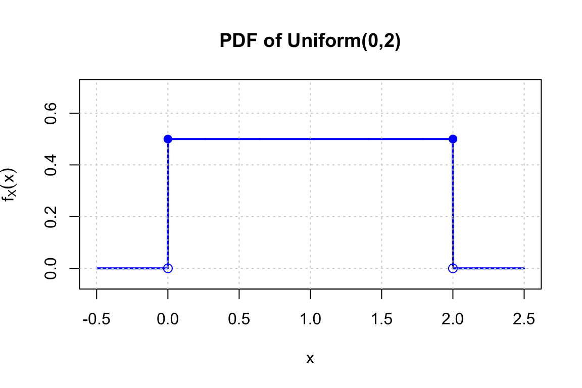
Therefore: \[ f_X(x) = \begin{cases} \frac{1}{2}, & 0 \leq x \leq 2\\ 0, & \text{otherwise} \end{cases} \]
Population Mean (using integral): \[\begin{align*} E(X) &= \int_{-\infty}^{\infty} x \cdot f_X(x)\,dx = \int_{0}^{2} x \cdot \frac{1}{2}\,dx\\ &= \frac{1}{2}\int_{0}^{2} x\,dx = \frac{1}{2}\left[\frac{x^2}{2}\right]_{0}^{2}\\ &= \frac{1}{2} \cdot \frac{4}{2} = \frac{1}{2} \cdot 2 = 1 \end{align*}\]
Variance (Method 1 - Direct Integration): \[\begin{align*} \text{Var}(X) &= \int_{-\infty}^{\infty} (x - \mu)^2 f_X(x)\,dx = \int_{0}^{2} (x - 1)^2 \cdot \frac{1}{2}\,dx\\ &= \frac{1}{2}\int_{0}^{2} (x^2 - 2x + 1)\,dx\\ &= \frac{1}{2}\left[\frac{x^3}{3} - x^2 + x\right]_{0}^{2}\\ &= \frac{1}{2}\left(\frac{8}{3} - 4 + 2\right) = \frac{1}{2}\left(\frac{8}{3} - 2\right)\\ &= \frac{1}{2} \cdot \frac{2}{3} = \frac{1}{3} \end{align*}\]
Variance (Method 2 - Using \(\text{Var}(X) = E(X^2) - [E(X)]^2\)):
First, compute \(E(X^2)\): \[\begin{align*} E(X^2) &= \int_{0}^{2} x^2 \cdot \frac{1}{2}\,dx = \frac{1}{2}\left[\frac{x^3}{3}\right]_{0}^{2}\\ &= \frac{1}{2} \cdot \frac{8}{3} = \frac{4}{3} \end{align*}\]
Then: \[\begin{align*} \text{Var}(X) &= E(X^2) - [E(X)]^2 = \frac{4}{3} - 1^2\\ &= \frac{4}{3} - 1 = \frac{1}{3} \end{align*}\]
Standard Deviation: \[ \sigma_X = \sqrt{\text{Var}(X)} = \sqrt{\frac{1}{3}} = \frac{1}{\sqrt{3}} = \frac{\sqrt{3}}{3} \approx 0.577 \]
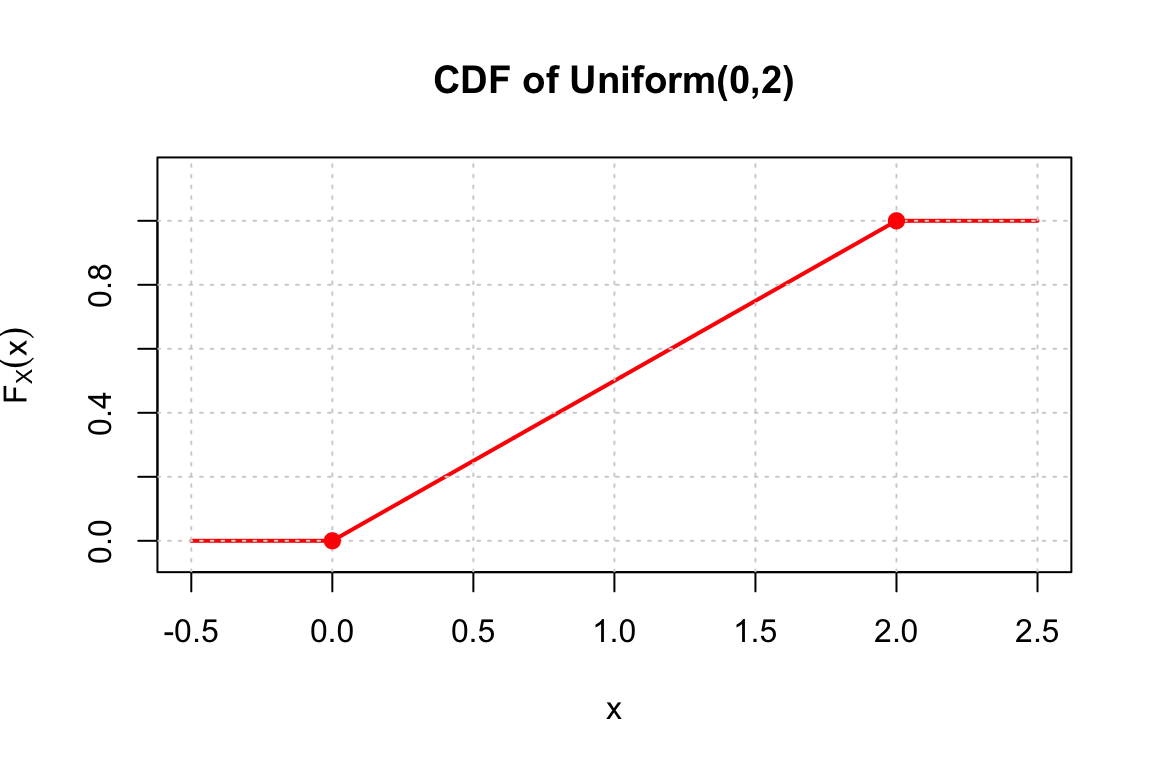
CDF: \[ F_X(x) = \begin{cases} 0, & x < 0\\ \frac{x-0}{2-0} = \frac{x}{2}, & 0 \leq x \leq 2\\ 1, & x > 2 \end{cases} \]
Quantile Function: For \(0 < q < 1\), solve \(F_X(\tau_{X,q}) = q\): \[ \frac{\tau_{X,q}}{2} = q \implies \tau_{X,q} = 2q \]
Median: \[ \text{Median} = \tau_{X,0.5} = 2(0.5) = 1 \]
PDF and CDF for Exercise 1
Applied Exercise 2
Problem: \(X\) is a continuous random variable with the following pdf: \[ f_X(x) = \begin{cases} ax, & -1 \leq x < 0\\ x, & 0 \leq x < 1\\ 0, & \text{otherwise} \end{cases} \] Determine the value of \(a\), the cdf \(F_X(x)\), the quantile function \(\tau_{X,q}\), and the population mean \(E(X)\).
Solution
Finding \(a\):
For a valid pdf, we need \(\int_{-\infty}^{\infty} f_X(x)\,dx = 1\): \[\begin{align*} \int_{-1}^{0} ax\,dx + \int_{0}^{1} x\,dx &= 1\\ a\left[\frac{x^2}{2}\right]_{-1}^{0} + \left[\frac{x^2}{2}\right]_{0}^{1} &= 1\\ a\left(0 - \frac{1}{2}\right) + \left(\frac{1}{2} - 0\right) &= 1\\ -\frac{a}{2} + \frac{1}{2} &= 1\\ -\frac{a}{2} &= \frac{1}{2}\\ a &= -1 \end{align*}\]
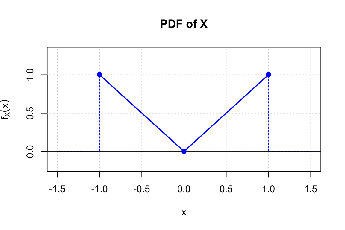
Therefore: \[ f_X(x) = \begin{cases} -x, & -1 \leq x < 0\\ x, & 0 \leq x < 1\\ 0, & \text{otherwise} \end{cases} \]
CDF \(F_X(x)\):
For \(x < -1\): \(F_X(x) = 0\)
For \(-1 \leq x < 0\): \[\begin{align*} F_X(x) &= \int_{-1}^{x} (-t)\,dt = -\left[\frac{t^2}{2}\right]_{-1}^{x}\\ &= -\frac{x^2}{2} + \frac{1}{2} = \frac{1-x^2}{2} \end{align*}\]
For \(0 \leq x < 1\): \[\begin{align*} F_X(x) &= \int_{-1}^{0} (-t)\,dt + \int_{0}^{x} t\,dt\\ &= \frac{1}{2} + \left[\frac{t^2}{2}\right]_{0}^{x} = \frac{1}{2} + \frac{x^2}{2} = \frac{1+x^2}{2} \end{align*}\]
For \(x \geq 1\): \(F_X(x) = 1\)
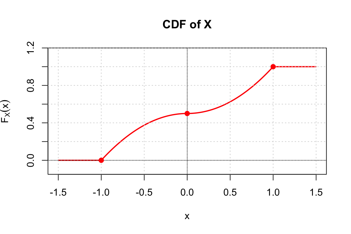
Therefore: \[ F_X(x) = \begin{cases} 0, & x < -1\\ \frac{1-x^2}{2}, & -1 \leq x < 0\\ \frac{1+x^2}{2}, & 0 \leq x < 1\\ 1, & x \geq 1 \end{cases} \]
Quantile Function \(\tau_{X,q}\):
For \(0 < q < 0.5\): Solve \(\frac{1-\tau_{X,q}^2}{2} = q\) \[\begin{align*} 1 - \tau_{X,q}^2 &= 2q\\ \tau_{X,q}^2 &= 1 - 2q\\ \tau_{X,q} &= -\sqrt{1-2q} \quad (\text{negative since } -1 \leq \tau_{X,q} < 0) \end{align*}\]
For \(0.5 \leq q < 1\): Solve \(\frac{1+\tau_{X,q}^2}{2} = q\) \[\begin{align*} 1 + \tau_{X,q}^2 &= 2q\\ \tau_{X,q}^2 &= 2q - 1\\ \tau_{X,q} &= \sqrt{2q-1} \quad (\text{positive since } 0 \leq \tau_{X,q} < 1) \end{align*}\]
Therefore: \[ \tau_{X,q} = \begin{cases} -\sqrt{1-2q}, & 0 < q < 0.5\\ \sqrt{2q-1}, & 0.5 \leq q < 1 \end{cases} \]
Population Mean \(E(X)\): \[\begin{align*} E(X) &= \int_{-1}^{0} x \cdot (-x)\,dx + \int_{0}^{1} x \cdot x\,dx\\ &= \int_{-1}^{0} (-x^2)\,dx + \int_{0}^{1} x^2\,dx\\ &= -\left[\frac{x^3}{3}\right]_{-1}^{0} + \left[\frac{x^3}{3}\right]_{0}^{1}\\ &= -\left(0 - \left(-\frac{1}{3}\right)\right) + \left(\frac{1}{3} - 0\right)\\ &= -\frac{1}{3} + \frac{1}{3} = 0 \end{align*}\]
PDF and CDF for Exercise 2
Applied Exercise 3
Problem: Random variables \(X\) and \(Y\) have the following joint pdf: \[ f_{XY}(x, y) = \begin{cases} axy, & 0 \leq x < y \leq 1\\ 0, & \text{otherwise} \end{cases} \] Determine: (a) the value of \(a\), (b) \(P(X \leq 2Y)\), (c) marginal pdf \(f_X(x)\), (d) \(E(X)\), (e) \(\text{Var}(X)\), (f) \(E(Y|X=0.5)\), and (g) check if \(X\) and \(Y\) are independent.
Solution
(a) Finding \(a\):
The region of integration is \(\{(x,y): 0 \leq x < y \leq 1\}\). \[\begin{align*} \int_{0}^{1}\int_{x}^{1} axy\,dy\,dx &= 1\\ a\int_{0}^{1} x\left[\frac{y^2}{2}\right]_{x}^{1}\,dx &= 1\\ a\int_{0}^{1} x\left(\frac{1}{2} - \frac{x^2}{2}\right)\,dx &= 1\\ \frac{a}{2}\int_{0}^{1} (x - x^3)\,dx &= 1\\ \frac{a}{2}\left[\frac{x^2}{2} - \frac{x^4}{4}\right]_{0}^{1} &= 1\\ \frac{a}{2}\left(\frac{1}{2} - \frac{1}{4}\right) &= 1\\ \frac{a}{2} \cdot \frac{1}{4} &= 1\\ a &= 8 \end{align*}\]
(b) Finding \(P(X \leq 2Y)\):
The condition \(X \leq 2Y\) is equivalent to \(Y \geq \frac{X}{2}\).
Given the constraint \(0 \leq x < y \leq 1\), we need \(y \geq \max(x, \frac{x}{2}) = x\) (since \(x > \frac{x}{2}\) for \(x > 0\)).
Therefore, \(X \leq 2Y\) is always satisfied in the support region, so: \[ P(X \leq 2Y) = 1 \]
(c) Marginal pdf \(f_X(x)\):
For \(0 \leq x \leq 1\): \[\begin{align*} f_X(x) &= \int_{x}^{1} 8xy\,dy = 8x\left[\frac{y^2}{2}\right]_{x}^{1}\\ &= 8x\left(\frac{1}{2} - \frac{x^2}{2}\right) = 4x(1 - x^2) \end{align*}\]
Therefore: \[ f_X(x) = \begin{cases} 4x(1-x^2), & 0 \leq x \leq 1\\ 0, & \text{otherwise} \end{cases} \]
(d) Expected Value \(E(X)\): \[\begin{align*} E(X) &= \int_{0}^{1} x \cdot 4x(1-x^2)\,dx = 4\int_{0}^{1} (x^2 - x^4)\,dx\\ &= 4\left[\frac{x^3}{3} - \frac{x^5}{5}\right]_{0}^{1} = 4\left(\frac{1}{3} - \frac{1}{5}\right)\\ &= 4 \cdot \frac{2}{15} = \frac{8}{15} \end{align*}\]
(e) Variance \(\text{Var}(X)\):
First, compute \(E(X^2)\): \[\begin{align*} E(X^2) &= \int_{0}^{1} x^2 \cdot 4x(1-x^2)\,dx = 4\int_{0}^{1} (x^3 - x^5)\,dx\\ &= 4\left[\frac{x^4}{4} - \frac{x^6}{6}\right]_{0}^{1} = 4\left(\frac{1}{4} - \frac{1}{6}\right)\\ &= 4 \cdot \frac{1}{12} = \frac{1}{3} \end{align*}\]
Therefore: \[\begin{align*} \text{Var}(X) &= E(X^2) - [E(X)]^2 = \frac{1}{3} - \left(\frac{8}{15}\right)^2\\ &= \frac{1}{3} - \frac{64}{225} = \frac{75}{225} - \frac{64}{225} = \frac{11}{225} \end{align*}\]
(f) Conditional Expected Value \(E(Y|X=0.5)\):
First, find the conditional pdf \(f_{Y|X}(y|x=0.5)\): \[ f_{Y|X}(y|x) = \frac{f_{XY}(x,y)}{f_X(x)} = \frac{8xy}{4x(1-x^2)} = \frac{2y}{1-x^2} \]
For \(x = 0.5\): \[ f_{Y|X}(y|0.5) = \frac{2y}{1-0.25} = \frac{2y}{0.75} = \frac{8y}{3}, \quad 0.5 < y \leq 1 \]
Then: \[\begin{align*} E(Y|X=0.5) &= \int_{0.5}^{1} y \cdot \frac{8y}{3}\,dy = \frac{8}{3}\int_{0.5}^{1} y^2\,dy\\ &= \frac{8}{3}\left[\frac{y^3}{3}\right]_{0.5}^{1} = \frac{8}{9}\left(1 - \frac{1}{8}\right)\\ &= \frac{8}{9} \cdot \frac{7}{8} = \frac{7}{9} \end{align*}\]
(g) Independence Check:
For independence, we need \(f_{XY}(x,y) = f_X(x) \cdot f_Y(y)\).
First, find \(f_Y(y)\). For \(0 \leq y \leq 1\): \[\begin{align*} f_Y(y) &= \int_{0}^{y} 8xy\,dx = 8y\left[\frac{x^2}{2}\right]_{0}^{y}\\ &= 8y \cdot \frac{y^2}{2} = 4y^3 \end{align*}\]
Now check: \(f_X(x) \cdot f_Y(y) = 4x(1-x^2) \cdot 4y^3 = 16xy^3(1-x^2)\)
This does not equal \(f_{XY}(x,y) = 8xy\).
Conclusion: \(X\) and \(Y\) are NOT independent.
Support Region for Exercise 3
The support region where \(f_{XY}(x,y) > 0\) is the triangular region defined by \(0 \leq x < y \leq 1\).
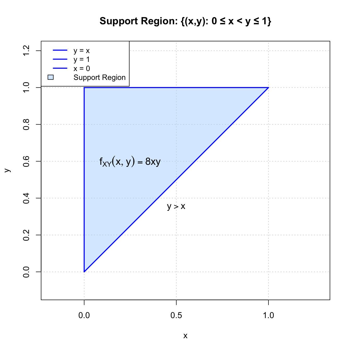
The shaded triangular region represents the area where the joint pdf is positive. The region is bounded by:
- Lower boundary: the line \(y = x\)
- Upper boundary: the line \(y = 1\)
- Left boundary: the line \(x = 0\)