Lab 01: Intro to R, Quarto

Author

Maghfira Ramadhani

Due date

This lab is due on Monday, September 15 at 11:59pm. To be considered on time, the following must be done by the due date:

Final .pdf file submitted on Gradescope

I’d recommend submitting ASAP, as most of today’s lab questions will be able to be done in class, spend your weekend prepping for midterm 1.

Introduction

The main goal is to introduce you to R and RStudio. We will use these throughout the course, both to learn the statistical concepts discussed in the lecture and to analyze real data and come to informed conclusions.

Note

R is the name of the programming language itself and RStudio is a convenient interface.

Learning goals

By the end of the lab, you will…

Be familiar with the workflow using RStudio
Gain practice writing a reproducible report using Quarto
Gain practice writing mathematical notation in (LaTeX) in Quarto.
Perform basic mathematical operations in R.
Write and read external from and to .csv in R.

Getting Started

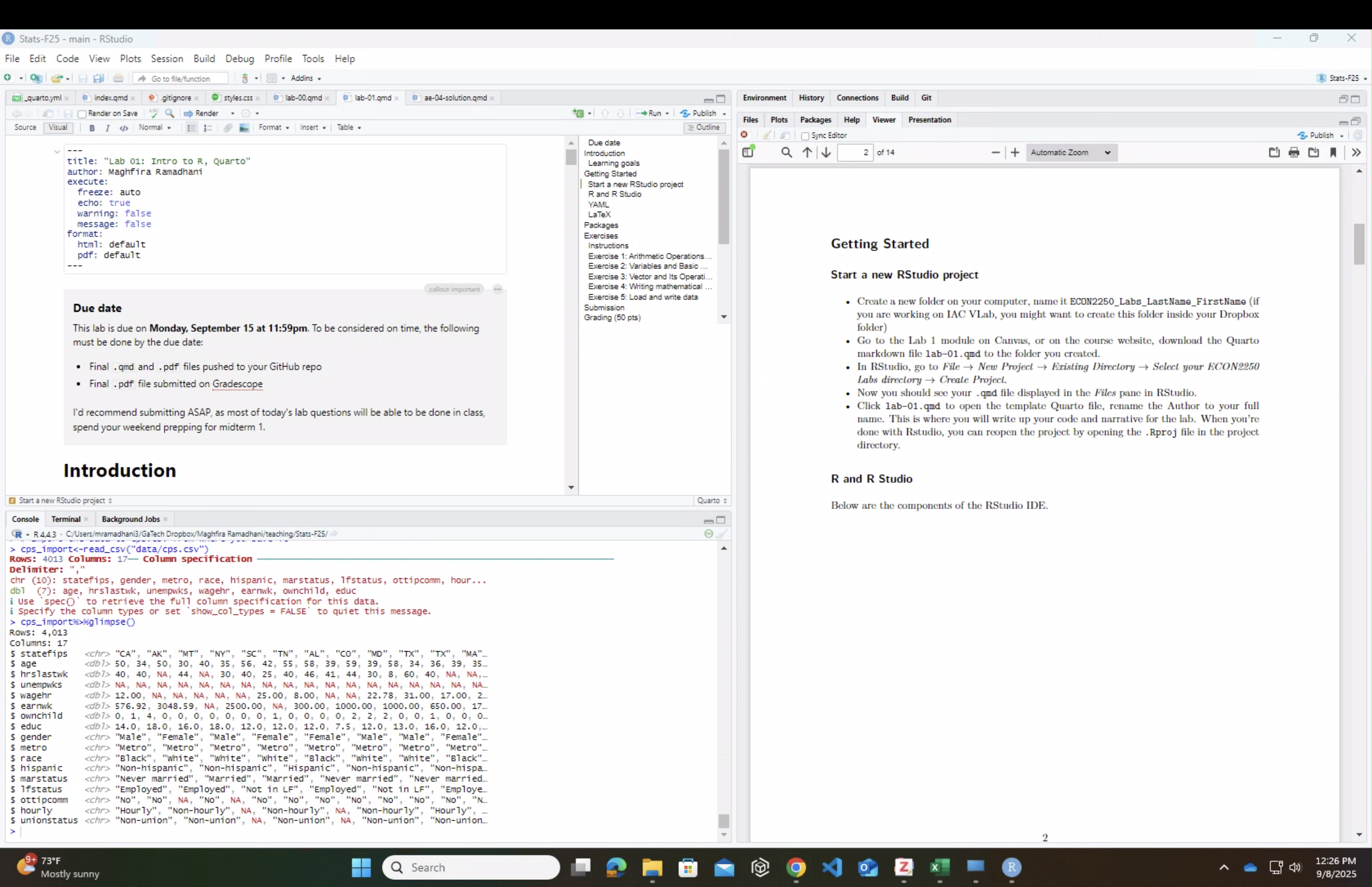
Start a new RStudio project

Create a new folder on your computer, name it ECON2250_Labs_LastName_FirstName (if you are working on IAC VLab, you might want to create this folder inside your Dropbox folder)
Go to the Lab 1 module on Canvas, or on the course website, download the Quarto markdown file lab-01.qmd to the folder you created.
In RStudio, go to File $\rightarrow$ New Project $\rightarrow$ Existing Directory $\rightarrow$ Select your ECON2250 Labs directory $\rightarrow$ Create Project.
Now you should see your .qmd file displayed in the Files pane in RStudio.
Click lab-01.qmd to open the template Quarto file, rename the Author to your full name. This is where you will write up your code and narrative for the lab. When you’re done with Rstudio, you can reopen the project by opening the .Rproj file in the project directory.

R and R Studio

Below are the components of the RStudio IDE:

Source Editor
Console
Environment -History - Git
Files - Plots - Packages - Help - Viewer

Below are the components of a Quarto (.qmd) file:

YAML
Code chunk
Narrative
Rendered output

Screenshot of Quarto document and rendered PDF.

YAML

The top portion of your Quarto file (between the three dashed lines) is called YAML. It stands for “YAML Ain’t Markup Language”. It is a human friendly data serialization standard for all programming languages. All you need to know is that this area is called the YAML (we will refer to it as such) and that it contains meta information about your document.

Important

Open the Quarto (.qmd) file in your project, change the author name to your name, and render the document. Examine the rendered document.

LaTeX

Quarto document uses LaTeX typesetting to write mathematical notation within the document. We will familiarize ourself with writing mathematical notation as we goes. Here are some example:

$x^2+y^2$ will render as $x^2+y^2$
$\sum_{i=1}^n x_i=\overline{x}$ will render as $\sum_{i=1}^n x_i=\overline{x}$

If you’re not sure how to write some mathematical notation in LaTeX, just ask.

Packages

A package is a collection of programs that someone else has written and published in public repository (basically a public goods). Package contain useful command or function so that we don’t have to code from scratch every time. We will need to install the package once before we can use it using install.packages("package1","package2"). We also need to load each package before we use them in our code using library(package1)

We will use the following packages in today’s lab.

library(probstats4econ)
library(tidyverse)
library(ggplot2)
library(knitr)

There’s a package manager named pacman that can handle the package installation for us

# load and install package if necessary
if (!require("pacman")) install.packages("pacman")
pacman::p_load(probstats4econ,tidyverse,ggplot2,knitr)

Exercises

Instructions

Write all code and narrative in your Quarto file. Write all narrative in complete sentences. Throughout the assignment, you should periodically render your Quarto document to produce the updated PDF.

Tip

Make sure we can read all of your code in your PDF document. This means you will need to break up long lines of code. One way to help avoid long lines of code is is start a new line after every pipe (|>) and plus sign (+).

Exercise 1: Arithmetic Operations and Mathematical Functions

Here are some mathematical operations in R:

7+8

[1] 15

7-8

[1] -1

7*8

[1] 56

7/8

[1] 0.875

7^8

[1] 5764801

1/3

[1] 0.3333333

R follows standard mathematical order of operations, which is in the following order from highest priority:

Parentheses$\rightarrow$Exponentiation$\rightarrow$Multiplication and Division$\rightarrow$Addition and substraction

Some commonly used mathematical functions are the following:

Calculates the absolute value $|x|$: abs(x)
Calculates the square root $\sqrt{x}$: sqrt(x)
Calculates the exponential value $e^x$: exp(x)
Calculates the natural logarightm $\ln{x}$: log(x) or use different base log(x,base=b)
Calculates the factorial $x!$: factorial(x)

Now perform the following exercise:

Compute the following calculation using R:
1. Add 9 by 29
2. Multiply 3 by 12
3. Calculates $(1+2^3)^2$.
4. Calculates $\log_{10} 1000$.
Write the code to compute the above quantity below:

# a
9+29
# b

# c

# d

Note

In this `lab-01.qmd` document you’ll see that we already added the code required for the exercise as well as a sentence where you can fill in the blanks to report the answer. Use this format for the remaining exercises.

Also note that the code chunk has a label: simple-math-operations. Labeling your code chunks is not required, but it is good practice and highly encouraged. Set eval: true if you want the program output to be printed in the PDF.

Exercise 2: Variables and Basic Operations

Most common data types in R are numeric, logical, character, date, factor.

x <- 1

x

x+5

x <- 2*x # Assign new value of x equal 2 times old x

x

rm(x) # Delete variable x

x # As we delete variable x, the program return error won't execute the next line of code

y <- 10.5

class(y) # Check types of variable y

y <- 10.5

class(y) # Check types of variable y

[1] "numeric"

str <- "ECON2250 Statistics for Economics"
class(str)

[1] "character"

Now perform the following exercise:

Create variables for the following economic indicators for the United States.
1. GDP : 25,000,000,000
2. Inflation Rate: 3.5%
3. Unemployment Rate: 4.2%
4. Population: 330 million

# GDP
GDP <- "___"
    
# Inflation_Rate
Inflation_Rate <- "___"
    
# Unemployment_Rate
Unemployment_Rate <- "___"

# Population
Population <- "__"

Use these variables to calculate the following:
1. GDP per capita
2. Unemployed individual in the US assuming labor force participation of 20%

# GDP_per_capita
GDP_per_capita <- "___"
GDP_per_capita    

# Unemployed_individuals
Unemployed_individuals <- "__"
Unemployed_individuals

Create the following character variables
1. Country: United States
2. Sector: Mixed

# Country
Country <- "___"
Country

# Sector
Sector <- "__"
Sector

Check the type of variable for each variable you created.

Exercise 3: Vector and Its Operations

A vector is a collection of elements of the same data type. The simplest method to create a vector is with the c function, and we can determine the length of a vector with the length function as follows:

# Define vector of numerics
numvec <- c(8,12,5,10,3)
numvec

[1]  8 12  5 10  3

numvec<-numvec^2
numvec

[1]  64 144  25 100   9

length(numvec)

[1] 5

# Define vector of characters
answers <- c("A","C","B","B","A","D")
answers

[1] "A" "C" "B" "B" "A" "D"

length(answers)

[1] 6

# Define vector of loficals
tfvec <- c(TRUE,FALSE,FALSE,TRUE)
tfvec

[1]  TRUE FALSE FALSE  TRUE

length(tfvec)

[1] 4

We can also create vector of numerics using seq(), :, or rep functions:

# Define vector of numerics 1,2,3,...,10
seq(1,10)

 [1]  1  2  3  4  5  6  7  8  9 10

seq(1,10,1)

 [1]  1  2  3  4  5  6  7  8  9 10

1:10

 [1]  1  2  3  4  5  6  7  8  9 10

# Define vector of zeros with length 5
rep(0,5)

[1] 0 0 0 0 0

# We can combine multiple vectors with c()
x<-c(1:10,rep(0,5))
x

 [1]  1  2  3  4  5  6  7  8  9 10  0  0  0  0  0

# We can acces i-th element of a vector
x[11]

[1] 0

# We can acces i-th to j-th element of a vector
x[1:5]

[1] 1 2 3 4 5

# We can acces select element of a vector
x[c(4,1,2)]

[1] 4 1 2

Commonly used vector-related functions are min(x), max(x), sort(x, decreasing=FALSE), unique(x), sum(x), mean(x), cumsum(x).

Now perform the following Exercise:

Create the following vectors.
1. Quarterly GDP Growth Rates: 1.8%, 2.0%, 1.75%, 1.9%
2. States: AL, AK, AZ, AR, CA

# Define Q_GDP_growth_rate
Q_GDP_growth_rate<- "__"
Q_GDP_growth_rate

# Define States
States<- "__"
States

Calculate the following using your vectors.
1. Minimum quarterly GDP growth rate
2. Average of GDP growth rates

# Compute the minimum of Q_GDP_growth_rate
Min_Q_GDP_growth_rate<- "__"
Min_Q_GDP_growth_rate

# Compute the average of Q_GDP_growth_rate
Mean_Q_GDP_growth_rate<- "__"
Mean_Q_GDP_growth_rate

Exercise 4: Writing mathematical notation

Having seen how mathematical notations are written so far, to complete these exercise, you just neet to type the formula for sample covariance and correlation below:

Sample covariance: \[\frac{Type your formula}{here}\]

Sample correlation: \[\sqrt{Type your formula here}\]

Exercise 5: Load and write data

We’re going to load the CPS data from the probstat4econ package.

library(probstats4econ)
cps%>%glimpse()

Rows: 4,013
Columns: 17
$ statefips   <fct> CA, AK, MT, NY, SC, TN, AL, CO, MD, TX, TX, MA, AZ, IL, WY…
$ age         <int> 50, 34, 50, 30, 40, 35, 56, 42, 55, 58, 39, 59, 39, 58, 34…
$ hrslastwk   <int> 40, 40, NA, 44, NA, 30, 40, 25, 40, 46, 41, 44, 30, 8, 60,…
$ unempwks    <int> NA, NA, NA, NA, NA, NA, NA, NA, NA, NA, NA, NA, NA, NA, NA…
$ wagehr      <dbl> 12.00, NA, NA, NA, NA, NA, 25.00, 8.00, NA, NA, 22.78, 31.…
$ earnwk      <dbl> 576.92, 3048.59, NA, 2500.00, NA, 300.00, 1000.00, 1000.00…
$ ownchild    <int> 0, 1, 4, 0, 0, 0, 0, 0, 0, 0, 1, 0, 0, 0, 0, 2, 2, 2, 0, 0…
$ educ        <dbl> 14.0, 18.0, 16.0, 18.0, 12.0, 12.0, 12.0, 7.5, 12.0, 13.0,…
$ gender      <fct> Male, Female, Male, Female, Female, Male, Male, Female, Fe…
$ metro       <fct> Metro, Metro, Metro, Metro, Metro, Metro, Metro, Metro, Me…
$ race        <fct> Black, White, White, White, Black, White, White, Black, Ot…
$ hispanic    <fct> Non-hispanic, Non-hispanic, Hispanic, Non-hispanic, Non-hi…
$ marstatus   <fct> Never married, Married, Married, Never married, Never marr…
$ lfstatus    <fct> Employed, Employed, Not in LF, Employed, Not in LF, Employ…
$ ottipcomm   <fct> No, No, NA, No, NA, No, No, No, No, No, No, No, No, No, No…
$ hourly      <fct> Hourly, Non-hourly, NA, Non-hourly, NA, Non-hourly, Hourly…
$ unionstatus <fct> Non-union, Non-union, NA, Non-union, NA, Non-union, Non-un…

cps%>%head()

  statefips age hrslastwk unempwks wagehr  earnwk ownchild educ gender metro
1        CA  50        40       NA     12  576.92        0   14   Male Metro
2        AK  34        40       NA     NA 3048.59        1   18 Female Metro
3        MT  50        NA       NA     NA      NA        4   16   Male Metro
4        NY  30        44       NA     NA 2500.00        0   18 Female Metro
5        SC  40        NA       NA     NA      NA        0   12 Female Metro
6        TN  35        30       NA     NA  300.00        0   12   Male Metro
   race     hispanic     marstatus  lfstatus ottipcomm     hourly unionstatus
1 Black Non-hispanic Never married  Employed        No     Hourly   Non-union
2 White Non-hispanic       Married  Employed        No Non-hourly   Non-union
3 White     Hispanic       Married Not in LF      <NA>       <NA>        <NA>
4 White Non-hispanic Never married  Employed        No Non-hourly   Non-union
5 Black Non-hispanic Never married Not in LF      <NA>       <NA>        <NA>
6 White Non-hispanic      Divorced  Employed        No Non-hourly   Non-union

Now we write the cps data locally to our computer

# Export the data to cps.csv in out project folder, 
# you can also write it into a subfolder "data"
write_csv(cps,"data/cps.csv")

Now to complete this exercise, you have to load the .csv and show the data below:

# Import the data to cps.csv from where you save it
cps_import<-read_csv("____")

# Show a glimpse of the data here

Submission

You will submit the PDF documents in to Gradescope as part of your final submission.

Warning

Remember – you must turn in a PDF file to the Gradescope page before the submission deadline for full credit.

Instructions to combine PDFs:

Preview (Mac): support.apple.com/guide/preview/combine-pdfs-prvw43696/mac
Adobe (Mac or PC): helpx.adobe.com/acrobat/using/merging-files-single-pdf.html

To submit your assignment:

Access Gradescope
Click on the assignment, and you’ll be prompted to submit it.
Mark the pages associated with each exercise. All of the pages of your lab should be associated with at least one question (i.e., should be “checked”).
Select the first page of your .PDF submission to be associated with the “Workflow & formatting” section.

Grading (50 pts)

This lab will be graded for completion, with each exercise worth 10 points. For example, if you complete all 5 exercises, you will receive a score of 50/50 for Lab 01. If you complete 3 exercises, you will receive a score of 30/50.

You will receive feedback on Lab 01, particularly if you have an error or an incomplete submission, as this is just an introduction to R.

You will receive feedback about “Workflow & formatting” for this lab, so you know what to expect for grading in future assignments. It will not count towards the grade in Lab 01.