Model of Discrete Random Variables
Week 7
Plan
In today’s class we will learn commonly used models for discrete random variables:
- Bernoulli random variables
- Binomial random variables
- Poisson random variables
Textbook Reference: JA 9.1, 9.2, 9.5; SDG 5.2, 5.4
Note that there are other models, e.g. Geometric, Hypergeometric, Negative Binomial, you can read them if you’re curious, but we won’t cover them in class (and won’t be tested).
A Clinical Trial
The treatment given to a particular patient in a clinical trial can either succeed or fail.
Let \(X=0\) if the treatment fails, and let \(X=1\) if the treatment succeeds.
All that is needed to specify the distribution of \(X\) is the value \(\pi=P(X=1)\).
Each different \(\pi\) corresponds to a different distribution for \(X\).
The collection of all such distribution corresponding to all \(0\leq\pi\leq1\) form the family of Bernoulli distributions.
Bernoulli random variables
A random variable \(X\) is a Bernoulli random variable with parameter \(\pi\) if \(X\in\{0,1\}\) and \(\pi=p_X(1)=P(X=1)\).
In math: \(X\sim \text{Bernoulli}(\pi)\)
In english: \(X\) has Bernoulli distribution with parameter \(\pi\).
Properties of Bernoulli r.v.
The p.f. of \(X\) can be written as \[p_X(x|\pi)=\begin{cases}p^x(1-p)^{1-x}&\text{for }x=0,1\\0& \text{otherwise.}\end{cases}\]
The population mean or expected value of \(X\) is: \[E(X)=1\cdot p + 0\cdot (1-p)=p.\]
The population variance of \(X\) is: \[\sigma_X^2=Var(X)=E[X^2-E(X)^2]=E(X^2)-E(X)^2=1^2\cdot p + 0^2\cdot (1-p)-p^2=p(1-p).\]
The population standard deviation of \(X\) is: \[\sigma_X=\sqrt{p(1-p)}\]
Bernoulli trials/process
If the random variables in a finite or infinite sequence \(X_1,X_2,\ldots\) are i.i.d (independent and identically distributed), and each \(X_i\sim\text{Bernoulli}(\pi)\), then we can say:
\(X_1,X_2,\ldots\) are Bernoulli trials/process with parameter \(\pi\).
Example:
Tossing a coin: \(X_i=1\) if head is obtained on the \(i\)-th toss, then \(X_1,X_2,\ldots\) are Bernoulli trials/process with parameter \(\pi=1/2\).
Clinical trials: \(X_i=1\) indicates whether patient \(i\) is a success, then \(X_1,X_2,\ldots\) are Bernoulli trials/process with parameter \(\pi=p\), where \(p\) is the unknown proportion of patients in a very large population who recover.
What if we define the number of head obtained or the number of patient succeed as a new random variables \(X\) such that \(X=X_1+X_2+\ldots+X_n\).
What is the distribution of \(X\)?
Binomial random variables
A random variable \(X\) is a Binomial random variable with parameter \(n\) and \(\pi\) if
\[X=X_1+X_2+\ldots+X_n\]
where \(X_1,X_2,\ldots,X_n\) are independent random variables with each \(X_i\sim\text{Bernoulli}(\pi)\).
Properties of Binomial r.v.
The p.f. of \(X\) can be written as \[p_X(x|n,\pi)=\begin{cases}\begin{pmatrix}n\\x\end{pmatrix}p^x(1-p)^{n-x}&\text{for }x=0,1,2,\ldots,n\\0& \text{otherwise.}\end{cases}\] (proof omitted for HW3)
The population mean or expected value of \(X\) is: \(E(X)=\sum_{i=1}^n E(X_i)=np.\)
The population variance of \(X\) is: \(\sigma_X^2=Var(X)=\sum_{i=1}^n Var(X_i)=np(1-p).\)
The population standard deviation of \(X\) is: \(\sigma_X=\sqrt{np(1-p)}.\)
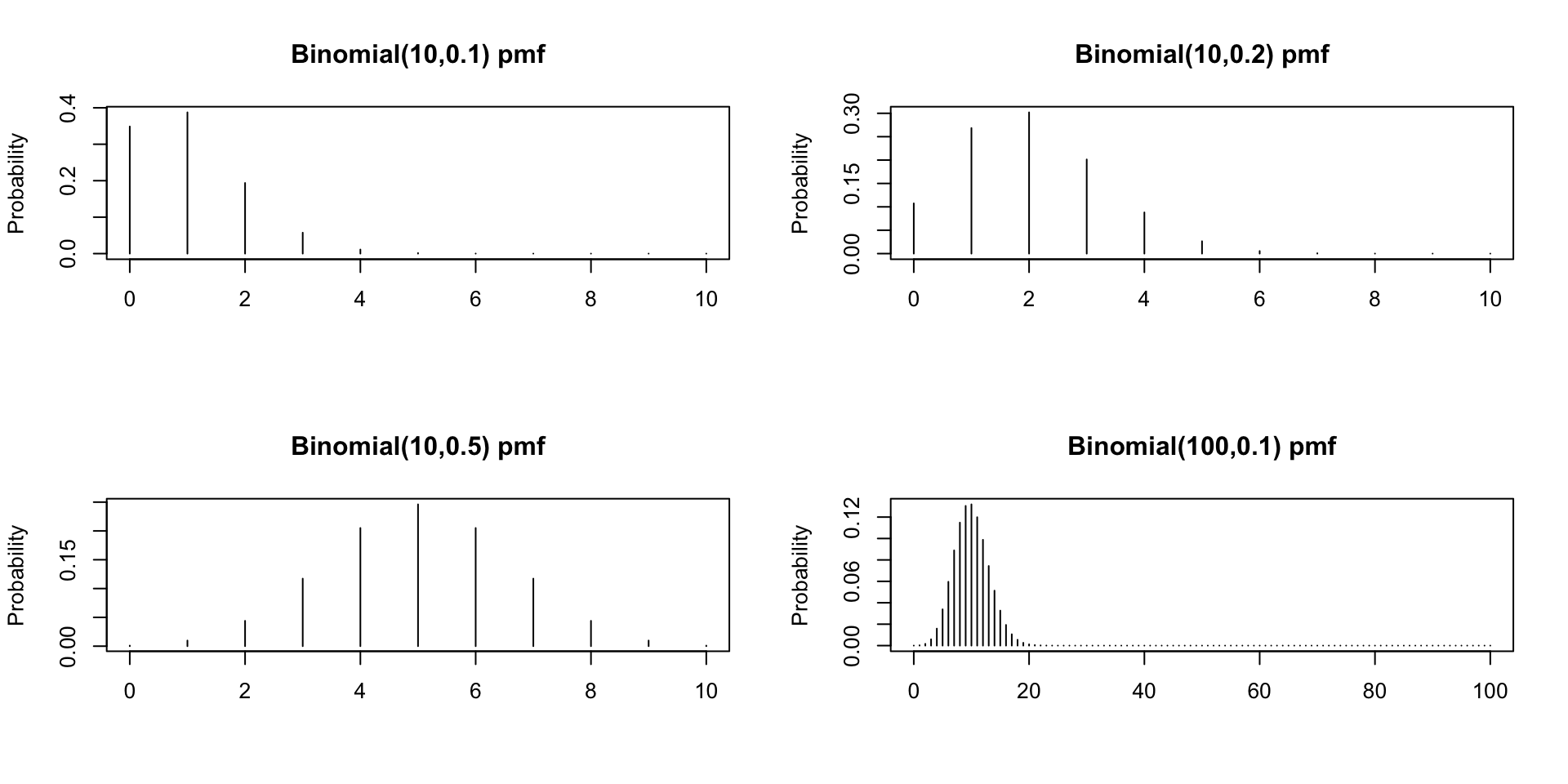
Example p.f. of binomial r.v.
Poisson random variables
A random variable \(X\) is a Poisson random variable with parameter \(\lambda>0\), if \(X\) represents the number of times that an event occurs within a fixed time interval and the following are true:
\(E(X)=\lambda\),
the average rate at which the event occur is constant (follow \(\lambda\)) and does not depent on whether previous events have occured,
the occurence of one event does not affect the likelihood that a future event occurs, and
two events cannot occur at exactly the same instant.
Range of possible outcome for \(X\sim\text{Poisson}(\lambda)\) are \(\{0,1,2,\ldots\}\)
Poisson random variables: Example
Consider a random variable \(X\) given as the number of customers who arrive at a coffee shop between 10 a.m. and 11 a.m. on a given weekday.
The expected value or population mean of \(X\) is 20. So, on average, a customer arrives every three minutes during the 10 a.m. to 11 a.m. hour.
For the assumptions of Poisson model to hold, it must be the case that:
the likelihood of one customer arriving has nothing to do with other customers arriving and
the likelihood of arrival is constant throughout the hour.
\(X∼\text{Poisson}(20).\)
Poisson random variables: Example
A firm has a research and development department that does research throughout the year.
Every so often, the department makes a discovery that leads to a patent application.
Let the random variable \(X\) be the number of discoveries (or patent applications) by the firm in a given year.
If the expected value of discoveries in a given year is equal to 2 and the research and development process satisfies the assumptions, then \(X∼\text{Poisson}(2)\).
Properties of Poisson r.v.
The p.f. of \(X\) can be written as \[p_X(x|\lambda)=\begin{cases}\frac{e^{-\lambda}\lambda^x}{x!}&\text{for }x=0,1,2,\ldots,\\0& \text{otherwise.}\end{cases}\]
The population mean or expected value of \(X\) is: \(E(X)=\lambda.\)
The population variance of \(X\) is: \(\sigma_X^2=\lambda.\)
The population standard deviation of \(X\) is: \(\sigma_X=\sqrt{\lambda}.\)
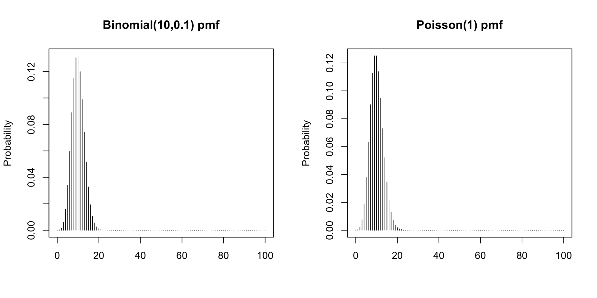
Poisson and Binomial
Poisson distribution are useful for approximating binomial distribution with very small success probabilities.