Rows: 4,013
Columns: 17
$ statefips   <fct> CA, AK, MT, NY, SC, TN, AL, CO, MD, TX, TX, MA, AZ, IL, WY…
$ age         <int> 50, 34, 50, 30, 40, 35, 56, 42, 55, 58, 39, 59, 39, 58, 34…
$ hrslastwk   <int> 40, 40, NA, 44, NA, 30, 40, 25, 40, 46, 41, 44, 30, 8, 60,…
$ unempwks    <int> NA, NA, NA, NA, NA, NA, NA, NA, NA, NA, NA, NA, NA, NA, NA…
$ wagehr      <dbl> 12.00, NA, NA, NA, NA, NA, 25.00, 8.00, NA, NA, 22.78, 31.…
$ earnwk      <dbl> 576.92, 3048.59, NA, 2500.00, NA, 300.00, 1000.00, 1000.00…
$ ownchild    <int> 0, 1, 4, 0, 0, 0, 0, 0, 0, 0, 1, 0, 0, 0, 0, 2, 2, 2, 0, 0…
$ educ        <dbl> 14.0, 18.0, 16.0, 18.0, 12.0, 12.0, 12.0, 7.5, 12.0, 13.0,…
$ gender      <fct> Male, Female, Male, Female, Female, Male, Male, Female, Fe…
$ metro       <fct> Metro, Metro, Metro, Metro, Metro, Metro, Metro, Metro, Me…
$ race        <fct> Black, White, White, White, Black, White, White, Black, Ot…
$ hispanic    <fct> Non-hispanic, Non-hispanic, Hispanic, Non-hispanic, Non-hi…
$ marstatus   <fct> Never married, Married, Married, Never married, Never marr…
$ lfstatus    <fct> Employed, Employed, Not in LF, Employed, Not in LF, Employ…
$ ottipcomm   <fct> No, No, NA, No, NA, No, No, No, No, No, No, No, No, No, No…
$ hourly      <fct> Hourly, Non-hourly, NA, Non-hourly, NA, Non-hourly, Hourly…
$ unionstatus <fct> Non-union, Non-union, NA, Non-union, NA, Non-union, Non-un…Data and Descriptive Statistics
Week 3 and 4
Maghfira Ramadhani
Sep 03, 2025
Plan
In today’s class we will discuss:
- Types of Data, Types of Variables, Sampling Methods
- Descriptive statistics and data visualizations
- Categorical data:
- Sample counts, sample proportions, sample mode, bar charts
- Numerical Data:
- Histograms
- Measure of location (sample mean, sample median, sample quantiles)
- Measure of dispersion (IQR, sample variance, sample std. dev.) (last class)
- Linear transformation and standardized values
- Bivariate Data:
- Scatterplot, Sample Covariance, and Correlation
- Categorical data:
Textbook Reference: JA Chapter 5-7
Types of Data
- Cross-sectional data
- Time-series data
- Panel (longitudinal) data
Cross-sectional data
Cross-sectional data consists of observations on different units that are measured at the same point in time or within the same time interval, or a “snapshot”.
The cross-sectional units can be individuals, households, firms, countries, states.
Cross-sectional data: Example
Labor-force data
| Individual | Period | Labor-force status | Earnings | Hours worked |
|---|---|---|---|---|
| 1 | 9/1/2025-9/7/2025 | Working | 700 | 55 |
| 2 | 9/1/2025-9/7/2025 | Unemployed | 0 | 0 |
| \[ \vdots \] | \[ \vdots \] | \[ \vdots \] | \[ \vdots \] | |
| 999 | 9/1/2025-9/7/2025 | Working | 500 | 40 |
Cross-sectional data: Example
State-level cigarette tax data
| State | Year | Cigarette taxes |
|---|---|---|
| GA | 2025 | 0.37 |
| NY | 2025 | 5.35 |
| \[ \vdots \] | \[ \vdots \] | \[ \vdots \] |
| NC | 2025 | 0.45 |
Time-series data
Time-series data consist of observations on the same unit that are measured at different points in time.
When the time series consists of a single variable, the data are univariate time-series data. When the time series consists of more than one variable, the data are multivariate time-series data.
Time-series data: Example
US macroeconomic indicators
| Year | Inflation rate | Gross domestic product |
|---|---|---|
| 2000 | 3.4 | 10,251.0 |
| 2001 | 2.8 | 10,581.9 |
| \[ \vdots \] | \[ \vdots \] | \[ \vdots \] |
| 2023 | 4.1 | 27,720.7 |
| 2024 | 2.9 | 29,184.9 |
Panel data
Panel (or longitudinal) data have both a cross-sectional dimension and a time-series dimension, with information about the same cross-sectional units being observed at different points in time.
The number of times that each cross-sectional unit is observed is at least two.
Panel data: Example
Firm’s revenue (in long panel format)
| Year | Firm | Revenue |
|---|---|---|
| 2000 | A | 10 |
| 2000 | B | 12 |
| 2001 | A | 9 |
| 2001 | B | 8 |
| \[ \vdots \] | \[ \vdots \] | \[ \vdots \] |
Panel data: Example
Firm’s revenue (in wide panel format)
| Firm | 2000 | 2001 | \[ \cdots \] |
|---|---|---|---|
| A | 10 | 9 | \[ \cdots \] |
| B | 12 | 8 | \[ \cdots \] |
Types of Variables
A variable is any measurable characteristic of a given unit of observation
There are two main types:
- Numerical variables
- Discrete variable: \(\{0,1,2,3,\ldots\}\)
- Continuous variable: \([0,\infty)\)
- Categorical variables
- Ordered: \(\{Jan,Feb,\ldots,Dec\},\ \{Very\ Bad, Bad, \ldots, Very\ Good\}\)
- Unordered: \(\{AL,AK,AZ,\ldots,WI,WV,WY\}\)
- Binary/Dummy/Indicator variable (1 or 0, Yes or No)
Random Sampling
- Recall week 1 intro materials about population and sample. The ideal version of a representative sample is known as a simple random sample.
- A sample of size \(n\) is called a simple random sample if each element of the population is equally likely to be sampled or, equivalently, that any possible sample of size \(n\) is equally likely to be chosen from the population.
- Any idea how to practically do it? What are the consequences for not random sampling?
- It may introduce sample selection bias
Stratified random sampling
- A stratified random sample is created by splitting the population into defined subpopulations or strata and drawing a simple random sample from each subpopulation or stratum.
- Such a sample is called a proportionate stratified random sample if the sizes of the strata samples are proportional to the true probabilities of the strata in the population, and a disproportionate stratified random sample if they are not.
- Why would one use proportionate or disproportionate stratified random sample?
Descriptive Statistics
Categorical data
For a categorical variable \(x\), with sample \(\{x_1,x_2,\ldots,x_n\}\), where there are \(C\) possible categories for \(x\).
We can describe the sample by
- the count of observations within each category \(c\in\{1,2,\ldots,C\}\), i.e. sample count, \[\text{sample count for category c}=\sum_{i=1}^n1(x_i=c)\]
- the fraction of observations within each category \(c\in\{1,2,\ldots,C\}\), i.e. sample proportion \[\text{sample proportion for category c}=\frac{\text{sample count for category c}}{n}\]
Categorical Data: Example
A subsample of the 2019 Current Population Survey (CPS)
Categorical Data: Example
A subsample of the 2019 Current Population Survey (CPS)
Categorical Data: Example
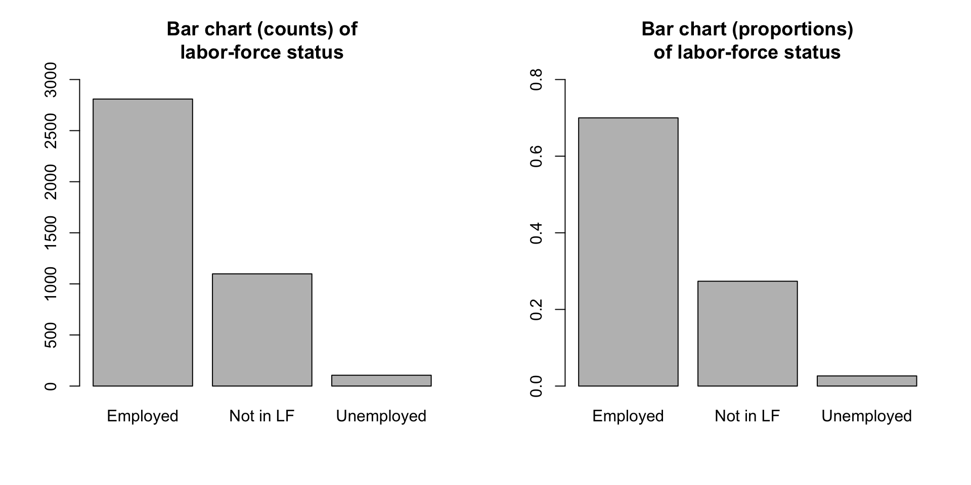
Sample count and sample proportion of 2019 CPS by labor force status
| Labor Force Status | Sample Count | Sample Proportion (%) |
|---|---|---|
| Employed | 2809 | 70.00 |
| Not in LF | 1098 | 27.36 |
| Unemployed | 106 | 2.64 |
| Total | 4013 | 100.00 |
Categorical Data: Example
Sample count and sample proportion of 2019 CPS by labor-force status
Numerical Data
There are a lot of ways to describe numerical data:
- Univariate:
- Histograms
- Measure of location (sample mean, sample median, sample quantiles)
- Measure of dispersion (IQR, sample variance, sample std. dev.)
- Bivariate (second variale could be categorical):
- Scatterplot
- Sample Covariance and Correlation
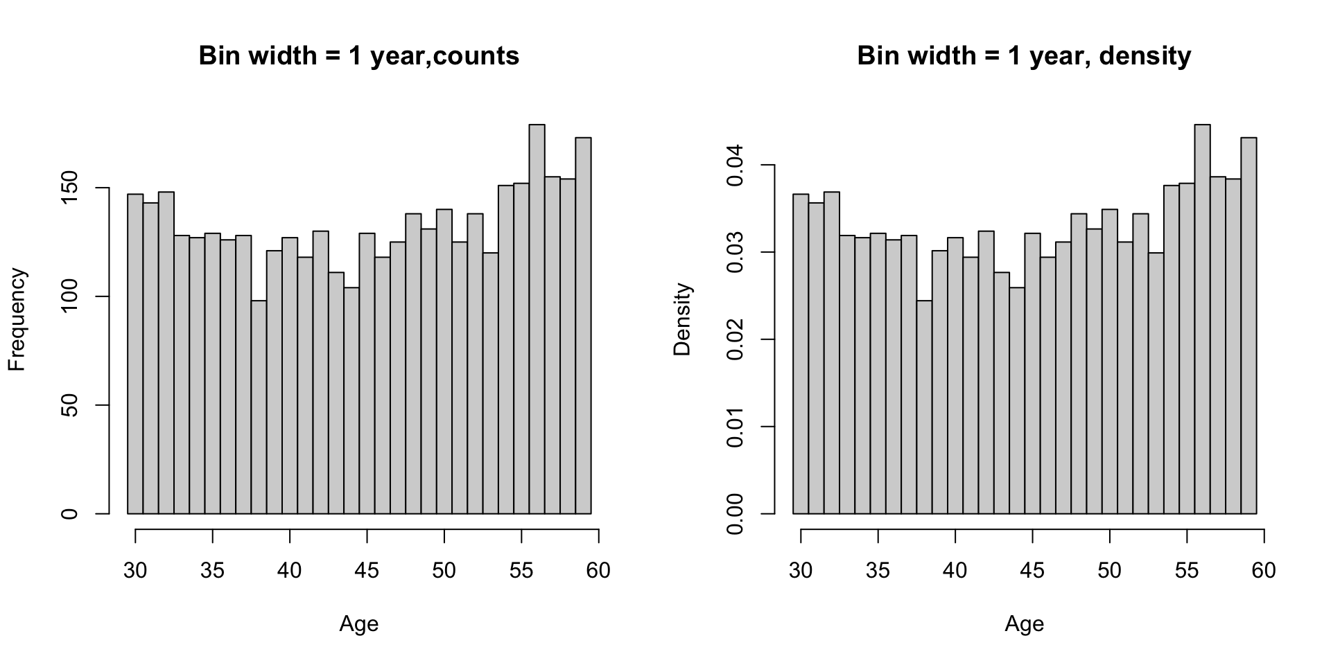
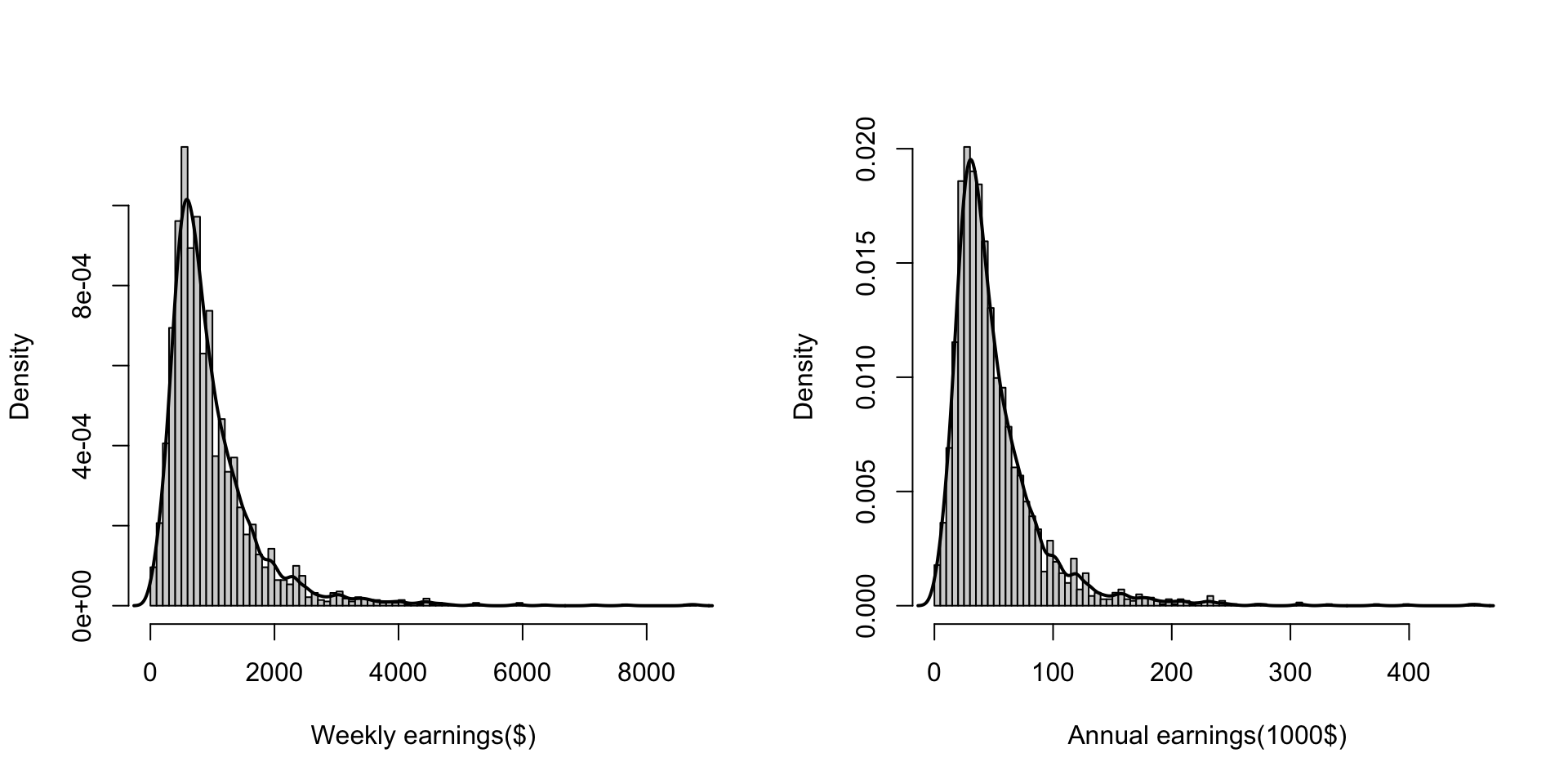
Histogram
2019 CPS age distribution
Histogram and Density
2019 CPS weekly earnings distribution of employed individuals
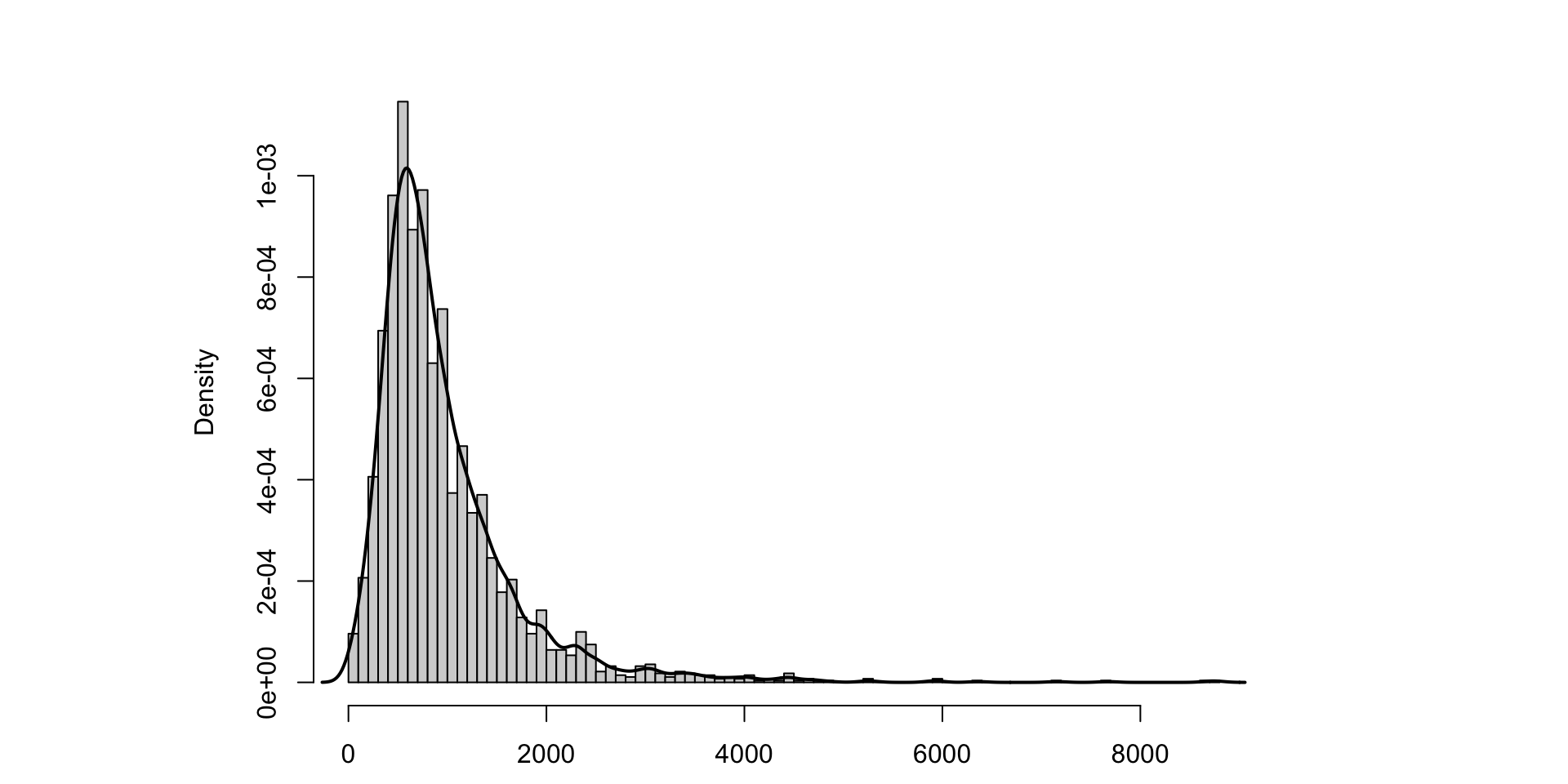
Bin-width selected follows Freedman-Diaconis rule of thumb: \(\text{bin width}=2\cdot\frac{{IQR}_x}{\sqrt[3]{n}}.\)
Measure of location
- Sample mean
- Sample quantiles
- Sample median
Sample mean
The sample mean of observation \(x_1,x_2,\ldots,x_n\) denoed as \(\overline{x}\), is \[ \overline{x}=\frac{x_1+x_2+\ldots+x_n}{n}=\frac{1}{n}\sum_{i=1}^n x_i. \]
Sample quantiles
For any \(q\) where \(0<q<1\), the sample quantiles, \(\tilde{x}_q\) is a value for which at least \(q\) fraction of the obserations are below (\(\leq\)) \(\tilde{x}_q\) and at least \(1-q\) fraction of the observations are above (\(\geq\)) \(\tilde{x}_q\).
Some special case:
- Sample median: \(\tilde{x}_{0.5}\)
- Sample quartiles: \(\tilde{x}_{q}\) where \(q\in\{0.25,0.5,0.75\}\)
- Sample deciles: \(\tilde{x}_{q}\) where \(q\in\{0.1,0.2,\ldots,0.9\}\)
- Sample percentiles: \(\tilde{x}_{q}\) where \(q\in\{0.01,0.02,\ldots,0.99\}\)
Sample quantiles details
Compute the sample quantiles for any value \(q\) from sample with \(n\) observation:
- Sort the observtion from lowest to highest.
- If \(nq\) is integer, then \(\tilde{x}_{q}\) is the average of the \(nq\)-th value and the \(nq+1\) value in the sorted sample. If \(nq\) is not integer, then \(\tilde{x}_{q}\) is the \(\lceil nq\rceil\)-th value (ceiling function: the smallest integer larger than)
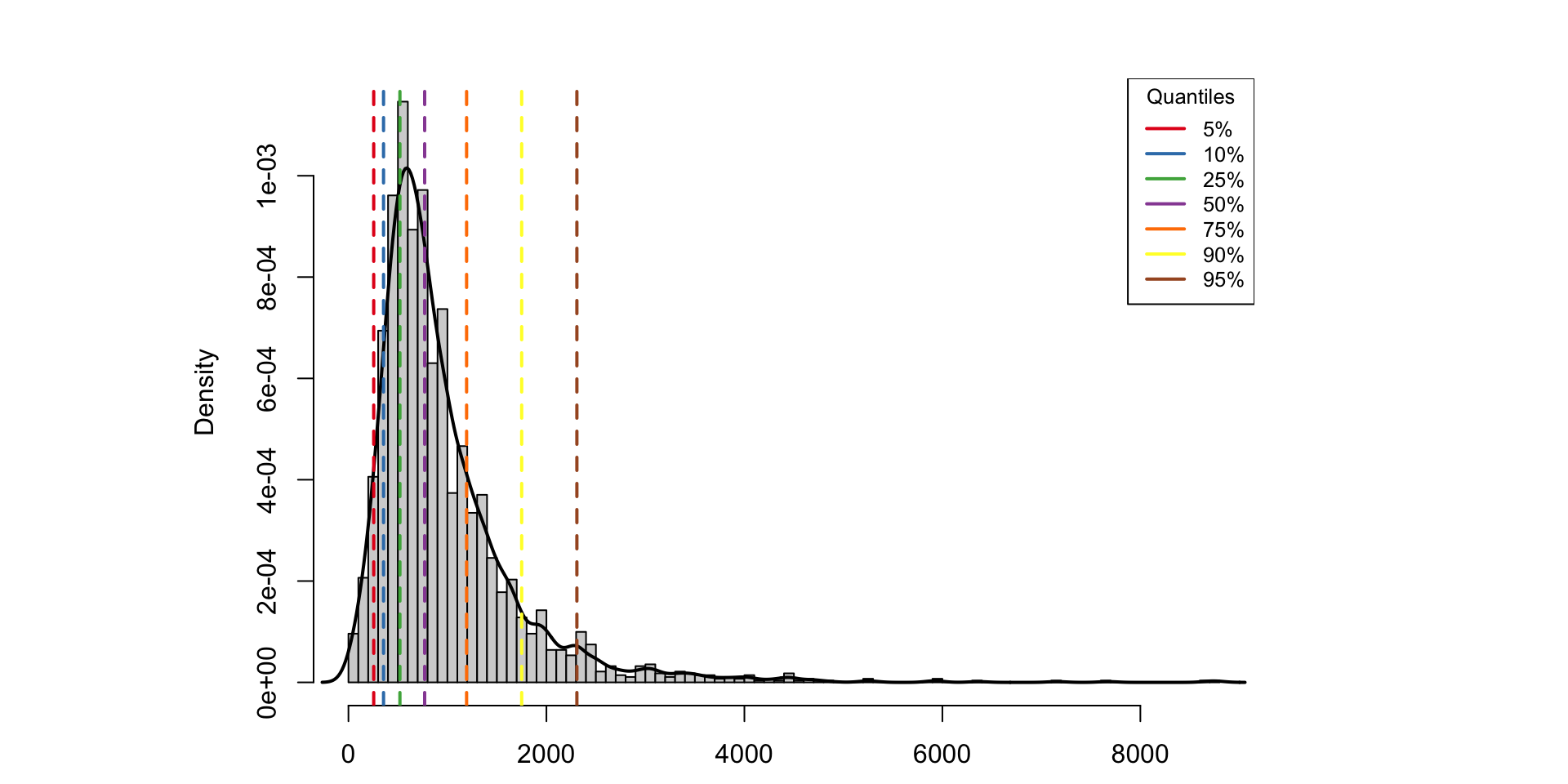
Sample quantiles: Example
2019 CPS weekly earnings quantiles
Sample quantiles: Example
2019 CPS weekly earnings quantiles
Measure of dispersion
- Interquartile range
- Sample mean absolute deviation
- Sample variance
- Sample standard deviation
Interquartile range
The range of observations \(x_1,x_2,x_3,\ldots,x_n\) is \[x_{max}-x_{min}.\]
The interquartile range (IQR) of observations \(x_1,x_2,x_3,\ldots,x_n\) is \[IQR_x=\tilde{x}_{0.75}-\tilde{x}_{0.25}.\]
Using boxplot to visualize dispersion
2019 CPS weekly earnings
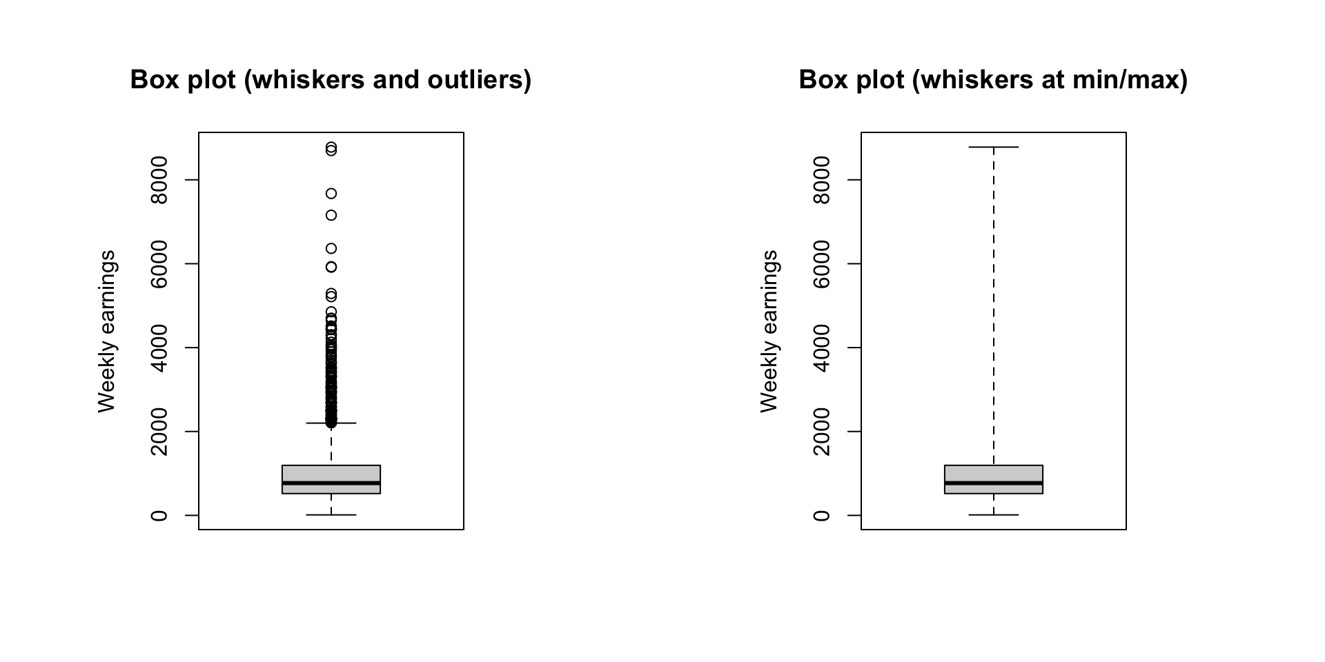
Outliers defined as being \(1.5IQR\) above the upper quartiles or \(1.5IQR\) below the lower quartiles
Sample mean absolute deviation
- Deviation from the mean: \(x_i-\overline{x}\)
- Sample mean absolute deviation: \[MAD_x=\frac{1}{n}\sum_{i=1}^n \lvert x_i-\overline{x}\rvert\]
Can be interpreted as average distance from the sample mean. The units of \(MAD_x\) is the same as the unit of \(x\).
Sample variance
The sample variance of observations \(x_1,x_2,x_3,\ldots,x_n\) is \[ s_x^2=\frac{1}{n-1}\sum_{i=1}^n (x_i-\overline{x})^2. \]
The units of \(s_x^2\) is the units of \(x\) squared.
Sample standard deviation
The sample standard deviation of observations \(x_1,x_2,x_3,\ldots,x_n\) is \[ s_x=\sqrt{s_x^2}=\sqrt{\frac{1}{n-1}\sum_{i=1}^n (x_i-\overline{x})^2}. \]
The units of \(s_x\) is similar to the units of \(x\).
Special cases, when \(x\in\{0,1\}\), the sample variance is \[s_x^2=\frac{n}{n-1}\overline{x}(1-\overline{x}).\]
Descriptive statistics: Example
2019 CPS Union vs Non-union worker’s wage
| Union Status | Sample Size (\(n\)) | Mean (\(\overline{x}\)) | MAD | Variance (\(s_x^2\)) | Std. Dev. (\(s_x\)) |
|---|---|---|---|---|---|
| Non-union | 2533 | 946.50 | 488.79 | 562120.3 | 749.75 |
| Union | 276 | 1197.65 | 532.42 | 518378.8 | 719.99 |
Descriptive statistics: Example
2019 CPS Male vs female worker’s wage
| Gender | Sample Size (\(n\)) | Mean (\(\overline{x}\)) | MAD | Variance (\(s_x^2\)) | Std. Dev. (\(s_x\)) |
|---|---|---|---|---|---|
| Female | 1308 | 803.49 | 415.14 | 457066.4 | 676.07 |
| Male | 1501 | 1117.30 | 529.94 | 610217.8 | 781.16 |
Plan
In today’s class we will discuss:
- Types of Data, Types of Variables, Sampling Methods
- Descriptive statistics and data visualizations
- Categorical data:
- Sample counts, sample proportions, sample mode, bar charts
- Numerical Data:
- Histograms
- Measure of location (sample mean, sample median, sample quantiles)
- Measure of dispersion (IQR, sample variance, sample std. dev.) (covered last class)
- Linear transformation and standardized values
- Bivariate Data:
- Scatterplot, Sample Covariance, and Correlation
- Categorical data:
Textbook Reference: JA Chapter 5-7
Modal outcome
The sample mode or modal outcome of observations \(x_1,x_2,\ldots,x_n\) is the value that occurs most often. It is possible that there is more than one sample mode, which happens when two or more outcomes are tied for being the most likely.
Modal outcome: Example 2019 CPS
Linear transformations
Sometimes we want to different variable that makes more economic sense than the original variable.
Can you think of examples where there’s would want to transform a variable?
Example:
- Units: Fahrenheit to Celcius, Inch to feet
- Economic variables: Profit=f(sales), annual earning=f(weekly earning)
If \(a\) and \(b\) are known constants, the variable \(y=a+bx\) is a linear transformation of the \(x\) variable. Moreover, the values \(y_i = a + b x_i (\text{for }i=1,\ldots,n)\) are linear transformations of the sample observations \(\{x_1,\ldots,x_n\}.\)
Linear transformations: Example annual earnings
Assume annual earnings (1000$)= 52 x weekly earnings ($)/1000, if weekly earning is \(x\) and annual earnings is \(y\), then \(y=0.052x\).
Descriptive statistics of the linear transformation
If \(a\) and \(b\) are known constants and \(y=a+bx\) is a linear transformation of \(x\), the descriptive statistics for the sample \(\{y_1,y_2,\ldots,y_n\}\) have the following relationships to the descriptive statistics for the sample \(\{x_1,x_2,\ldots,x_n\}\):
- Sample mean: \(\overline{y}=a+b\overline{x}\)
- Sample variance: \(s_y^2=b^2s_x^2\)
- Sample s.d.: \(s_y=|b|s_x\)
- Sample quantiles: \(\tilde{y}_q=a+b\tilde{x}_q\) if \(b\geq0\)
- Sample IQR: \(IQR_y=|b|IQR_x\) if \(b\geq0\)
- Sample MAD: \(MAD_y=|b|MAD_x\)
Linear transformations: Example annual earnings
Assume annual earnings (1000$)= 52 x weekly earnings ($)/1000, if weekly earning is \(x\) and annual earnings is \(y\), then \(y=0.052x\). Annual earnings are linear transformation of weekly earnings, with \(a=0,b=0.012\).
The followings are true:
- Sample mean: \(\overline{y}=0.052\overline{x}\)
- Sample variance: \(s_y^2=(0.052)^2s_x^2=0.0027s_x^2\)
- Sample s.d.: \(s_y=0.052s_x\)
- Sample quantiles: \(\tilde{y}_q=0.052\tilde{x}_q\)
- Sample IQR: \(IQR_y=0.052IQR_x\)
- Sample MAD: \(MAD_y=0.052MAD_x\)
Standardized value
It can be difficult to compare variables that have different means, variances, and different units, a commonly used linear transformation is the standardized values.
Standardized values of \(x_i\) is given by \[y_i=\frac{x_i-\overline{x}}{s_x}.\] It is a special case of linear transformation with \(a=-\overline{x}/s_x,b=1/s_x\)
After demeaning, the standardized value will have sample mean of zero (\(\overline{y}\)) and sample s.d. of one (\(s_y=1\)).
Example:
- Z-scores standardize test scores to compare student performance across schools or regions, adjusting for different grading scales.
- In randomized control trials, z-scores measure changes in learning outcomes, assessing the effectiveness of new teaching methods or curricula.
Descriptive statistics of multivariate data
- Joint sample counts or joint sample proportion
- (Again) Bar chart and box plot
- Scatterplot
- Sample covariance and correlation
Joint sample counts or proportion
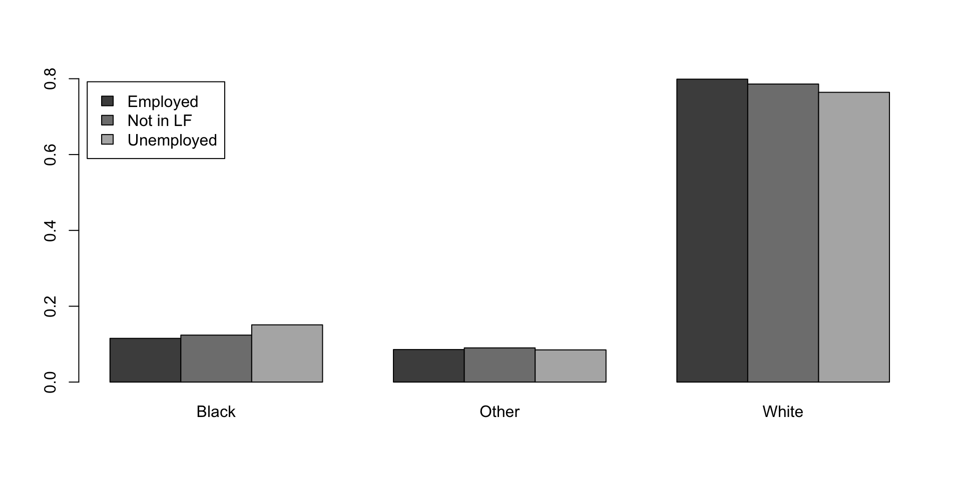
Joint sample count for labor-force status and race
| Black | Other | White | Sum | |
|---|---|---|---|---|
| Employed | 324 | 241 | 2244 | 2809 |
| Not in LF | 136 | 99 | 863 | 1098 |
| Unemployed | 16 | 9 | 81 | 106 |
| Sum | 476 | 349 | 3188 | 4013 |
Joint sample counts or proportion
Joint Sample proportion for labor-force status and race
| Black | Other | White | Sum | |
|---|---|---|---|---|
| Employed | 0.081 | 0.060 | 0.559 | 0.700 |
| Not in LF | 0.034 | 0.025 | 0.215 | 0.274 |
| Unemployed | 0.004 | 0.002 | 0.020 | 0.026 |
| Sum | 0.119 | 0.087 | 0.794 | 1.000 |
Joint sample counts or proportion
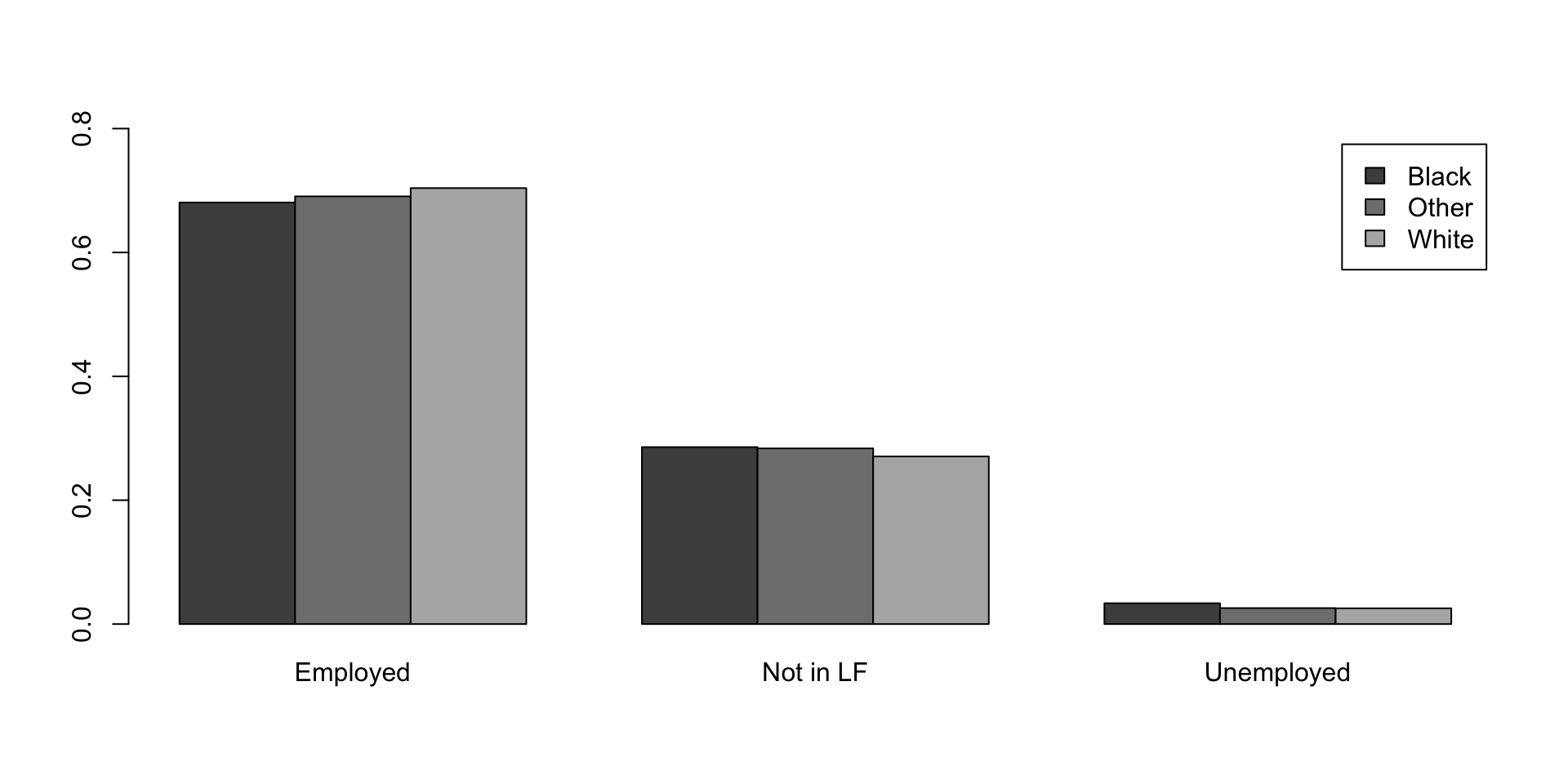
Sample proportions of labor-force status conditional on race
| Black | Other | White | |
|---|---|---|---|
| Employed | 0.681 | 0.691 | 0.704 |
| Not in LF | 0.286 | 0.284 | 0.271 |
| Unemployed | 0.034 | 0.026 | 0.025 |
Joint sample counts or proportion
Sample proportions of race conditional on labor-force status
| Black | Other | White | |
|---|---|---|---|
| Employed | 0.115 | 0.086 | 0.799 |
| Not in LF | 0.124 | 0.090 | 0.786 |
| Unemployed | 0.151 | 0.085 | 0.764 |
Bar charts: Labor-force status proportions by race
Bar charts: Race proportions by labor-force status
Showing distribution for different category
Box plots of weekly earnings by race
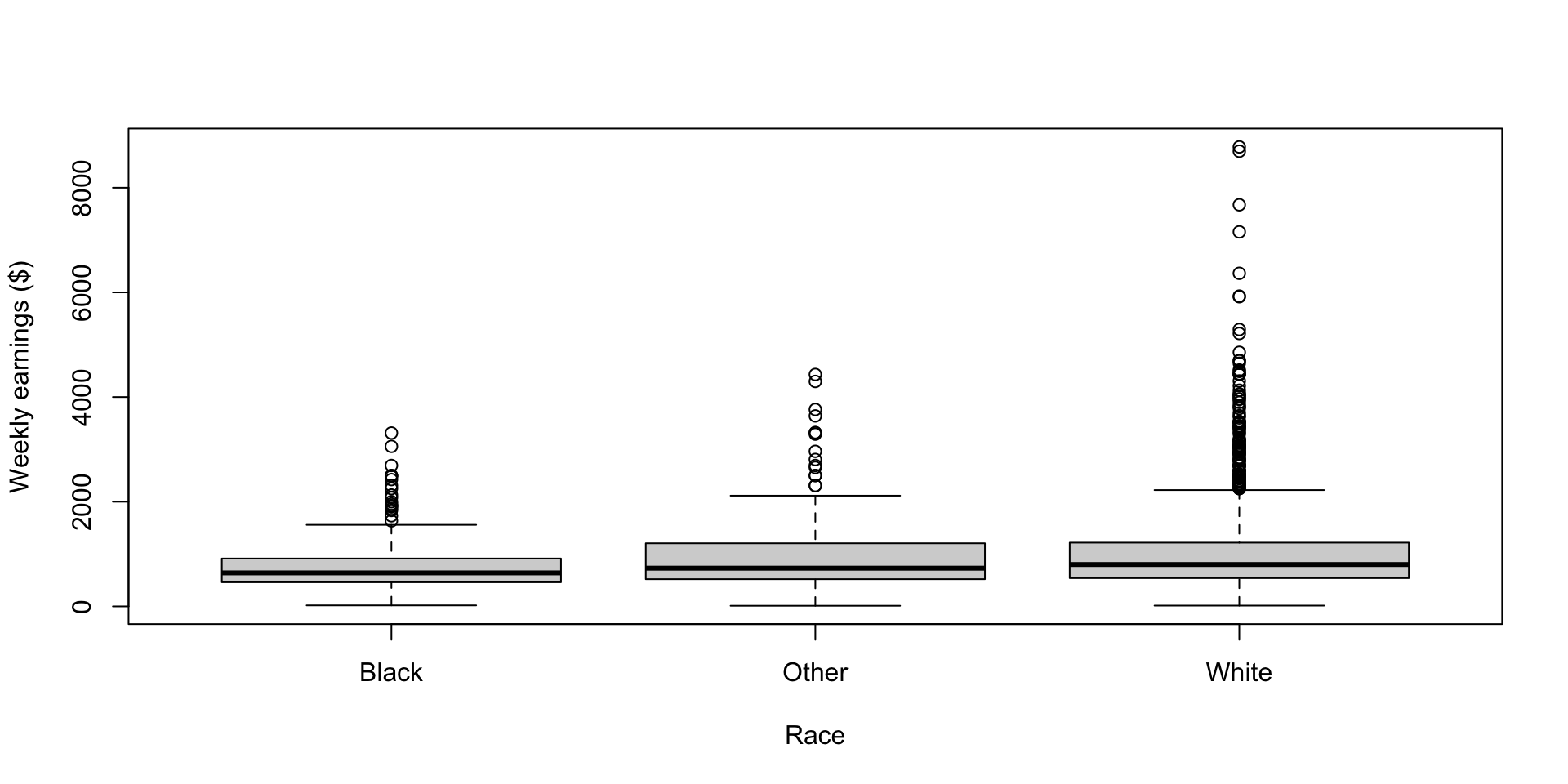
Showing distribution for different category
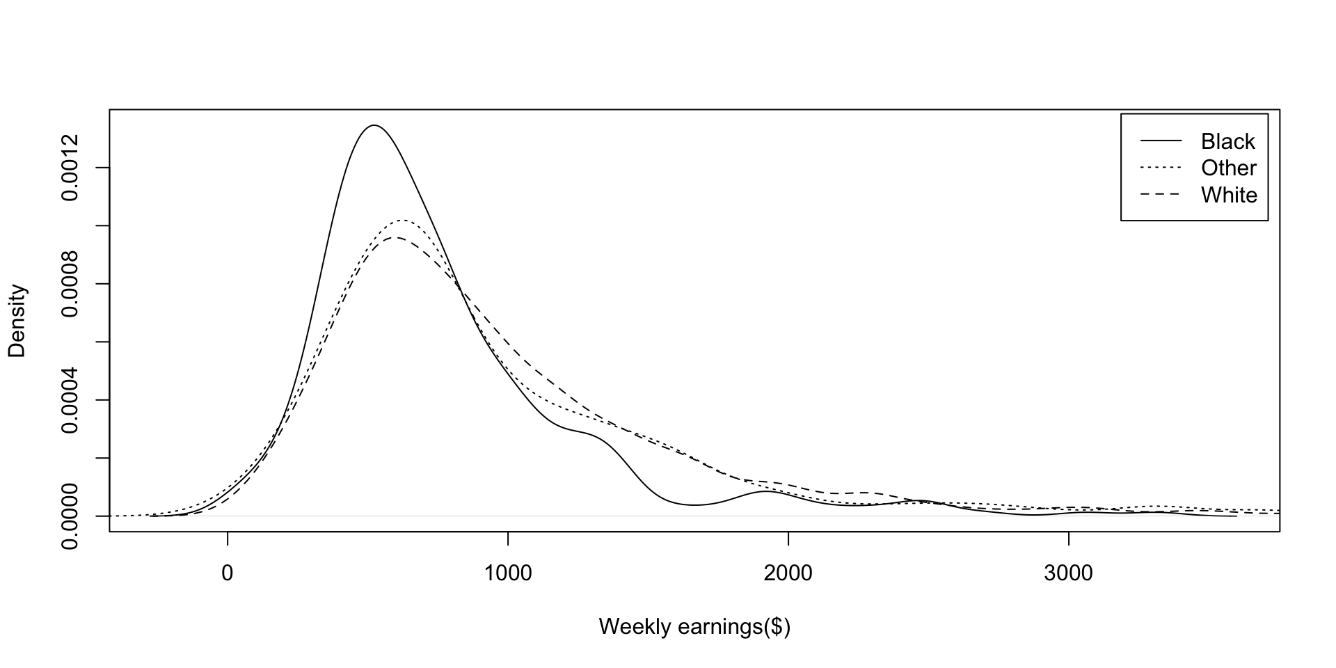
Density of weakly earnings by race
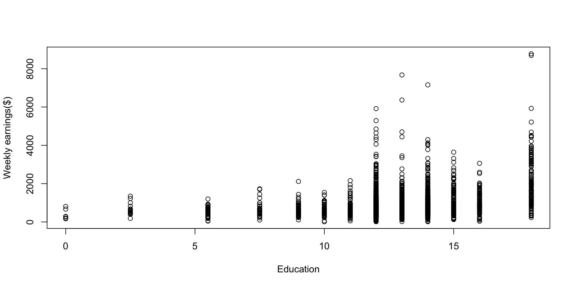
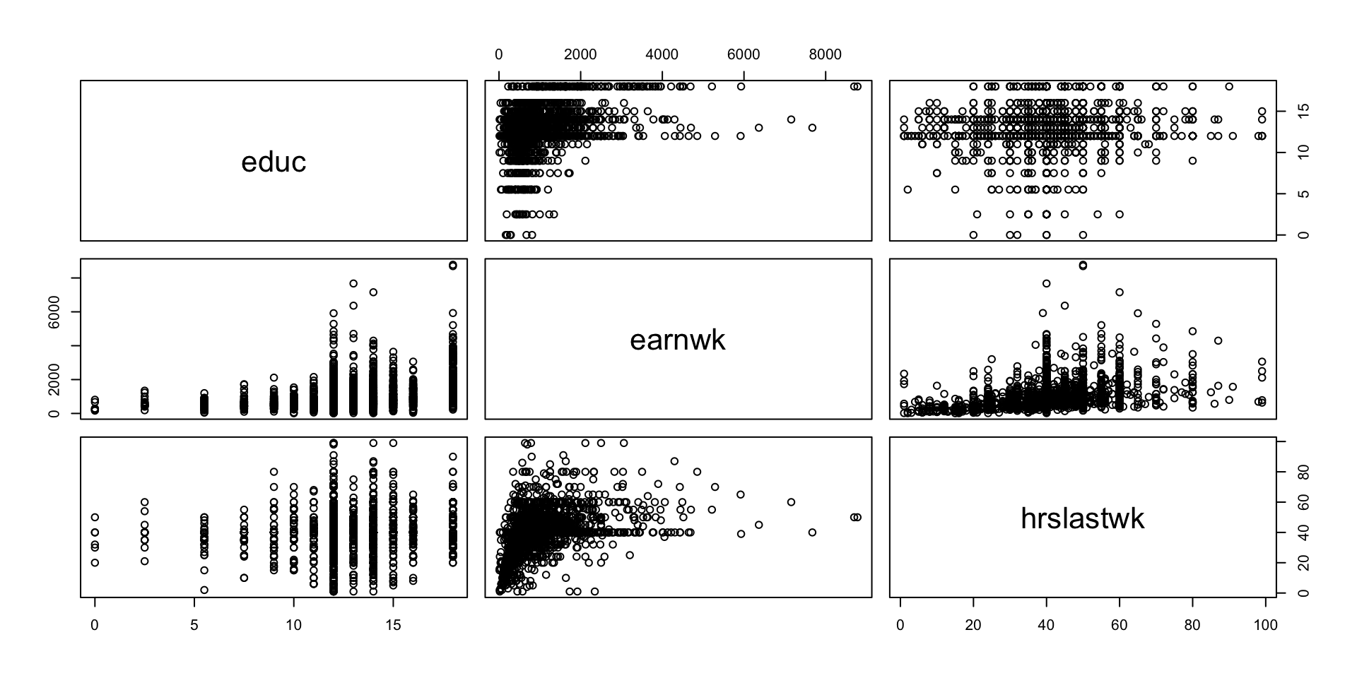
Scatterplot: visualizing bivariate numerical data
Weekly earnings versus years of education
Expanded scatterplot: visualizing multiple pairs of numerical data
Weekly earnings vs years of education vs weekly hours worked
Descriptive statistics: Relationship of two numerical variables
We’ve seen scatter plots provide a visualization of relationship between two numerical variables.
There are two descriptive statistics that can be used to describe these relationships:
- Sample covariance denoted \(s_{xy}\).
- Sample correlation denoted \(r_{xy}\).
Sample covariance
Sample covariance denoted \(s_{xy}\) is given by: \[ s_{xy}=\frac{1}{n-1}\sum_{i=1}^n (x_i-\overline{x})(y_i-\overline{y}). \] Note that sample variance \(s_{xx}\) is a special case of sample covariance: \[ s_x^2=s_{xx}=\frac{1}{n-1}\sum_{i=1}^n (x_i-\overline{x})(x_i-\overline{x}).\]
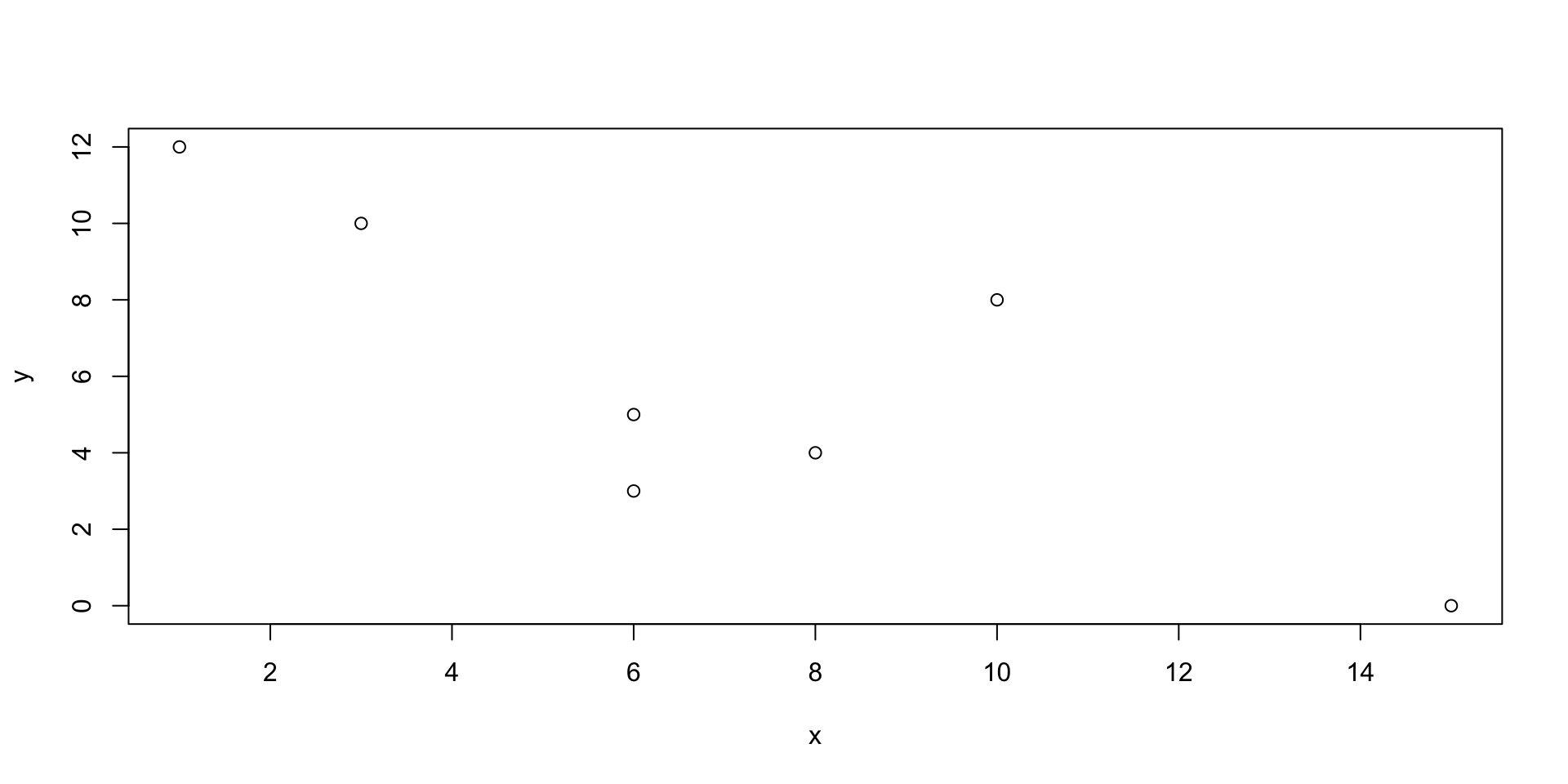
Sample covariance: Example
Consider the following data with n=7.
| \[ i \] | 1 | 2 | 3 | 4 | 5 | 6 | 7 |
| \[ x_i \] | 4 | 3 | 8 | 12 | 0 | 10 | 5 |
| \[ y_i \] | 8 | 6 | 10 | 1 | 15 | 3 | 6 |
Sample covariance: Example
Here’s the scatter plot of the data, what relationship do you see?
Sample covariance: Example
First, compute the mean: \(\overline{x}=\ldots, \overline{y}=\ldots\)
| \[ i \] | 1 | 2 | 3 | 4 | 5 | 6 | 7 |
| \[ x_i \] | 4 | 3 | 8 | 12 | 0 | 10 | 5 |
| \[ y_i \] | 8 | 6 | 10 | 1 | 15 | 3 | 6 |
| \[ x_i-\overline{x} \] | |||||||
| \[ y_i-\overline{y} \] | |||||||
| \[ (x_i-\overline{x})(y_i-\overline{y}) \] |
Sample covariance: Example
Then, using the mean \(\overline{x}=6, \overline{y}=7\), compute \(x_i-\overline{x}\) and \(y_i-\overline{y}\)
| \[ i \] | 1 | 2 | 3 | 4 | 5 | 6 | 7 |
| \[ x_i \] | 4 | 3 | 8 | 12 | 0 | 10 | 5 |
| \[ y_i \] | 8 | 6 | 10 | 1 | 15 | 3 | 6 |
| \[ x_i-\overline{x} \] | -2 | -3 | 2 | 6 | -6 | 4 | -1 |
| \[ y_i-\overline{y} \] | 1 | -1 | 3 | -6 | 8 | -4 | -1 |
| \[ (x_i-\overline{x})(y_i-\overline{y}) \] |
Sample covariance: Example
Then, compute \((x_i-\overline{x})(y_i-\overline{y})\)
| \[ i \] | 1 | 2 | 3 | 4 | 5 | 6 | 7 |
| \[ x_i \] | 4 | 3 | 8 | 12 | 0 | 10 | 5 |
| \[ y_i \] | 8 | 6 | 10 | 1 | 15 | 3 | 6 |
| \[ x_i-\overline{x} \] | -2 | -3 | 2 | 6 | -6 | 4 | -1 |
| \[ y_i-\overline{y} \] | 1 | -1 | 3 | -6 | 8 | -4 | -1 |
| \[ (x_i-\overline{x})(y_i-\overline{y}) \] | -2 | +3 | +6 | -36 | -48 | -16 | +1 |
Sample covariance: Example
Finally, compute the sample covariance: \[s_{xy}=\frac{1}{7-1}(-92)\approx -15.33.\] If we plot the means in the scatterplot, can we intuitively guess the sign of the covarience?

Sample covariance: Example
Scatter plot of weekly earnings vs education

- Can you guess the sign of the sample covariance?
- The sample covariance is 586.375 years\(\times\)dollars (note the unit)
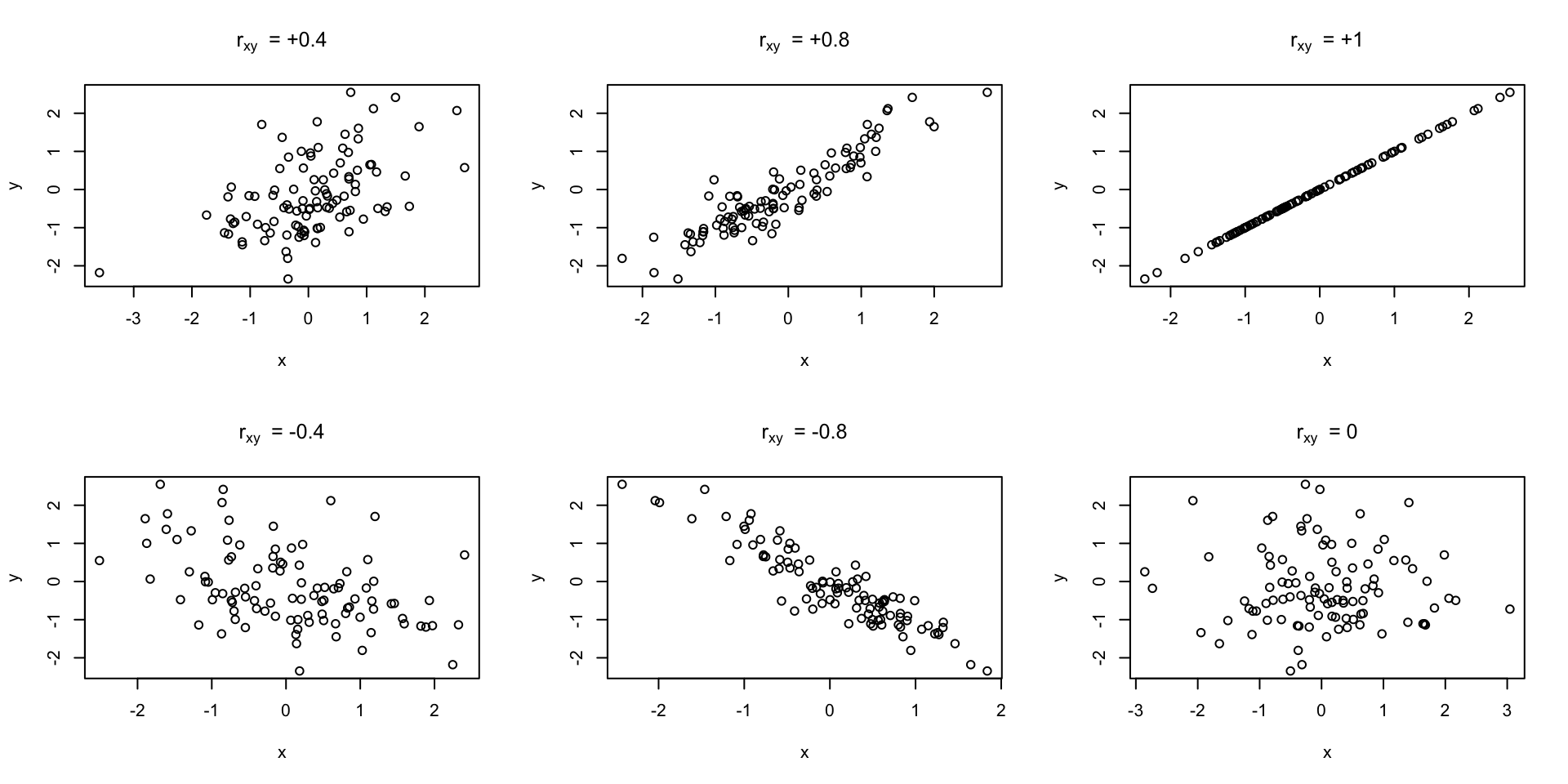
Sample correlation
Sample correlation also measures the linear association between two variables in a way that is comparable across different pairs of variables
Sample correlation between \(x\) and \(y\) is given by \[ r_{xy}=\frac{s_{xy}}{s_x s_y}, \] where \(s_{xy}\) is the sample covariance, \(s_x\) is the sample s.d. of \(x\), and \(s_y\) is the sample s.d. of \(y\).
Sample correlation \(r_{xy}\) has the following properties:
- is unitless
- has the same sign as the sample covariance
- \(r_{xx}\)=1
- \(-1\leq r_{xy}\leq 1\).
Scatter plot for different sample correlation
Caveat for sample correlation
Sample correlation only meant to measure linear association, when the relationship is not linear, it might not detect non-linear relationship.
Example of data with a sample correlation of zero
Sample correlation:[1] 2.537653e-15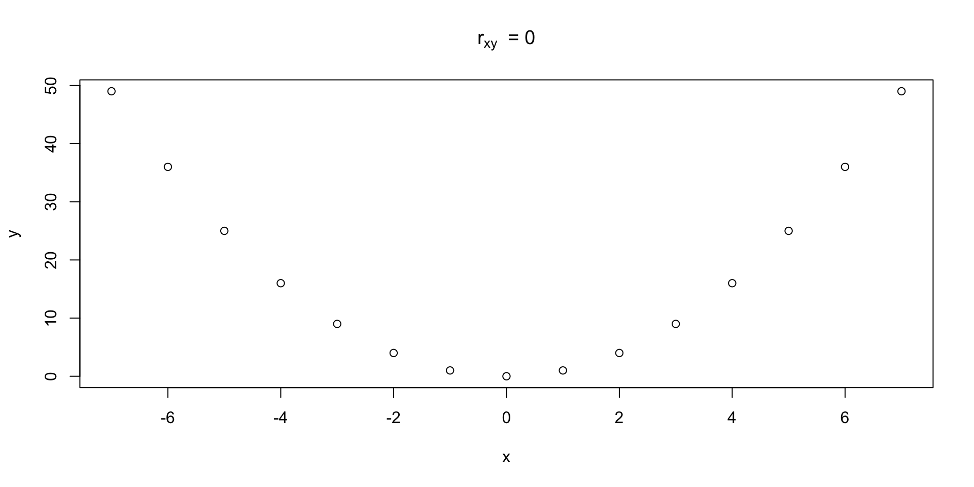
Caveat for sample correlation
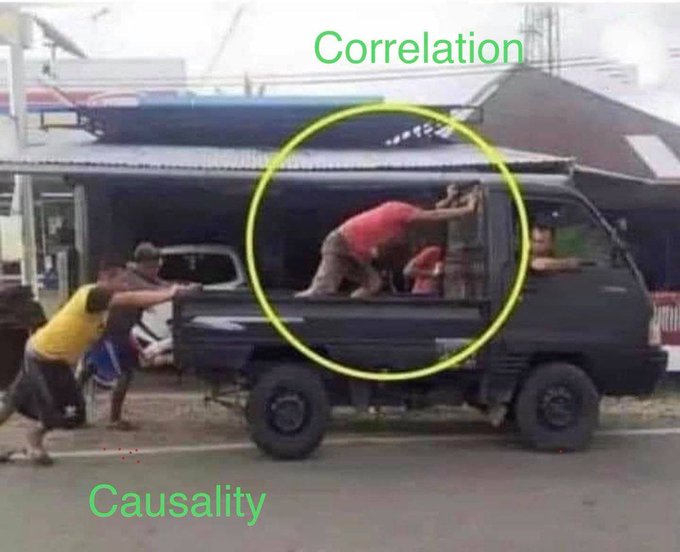
Correlation is not causation
Scatter plot of weekly earnings vs education
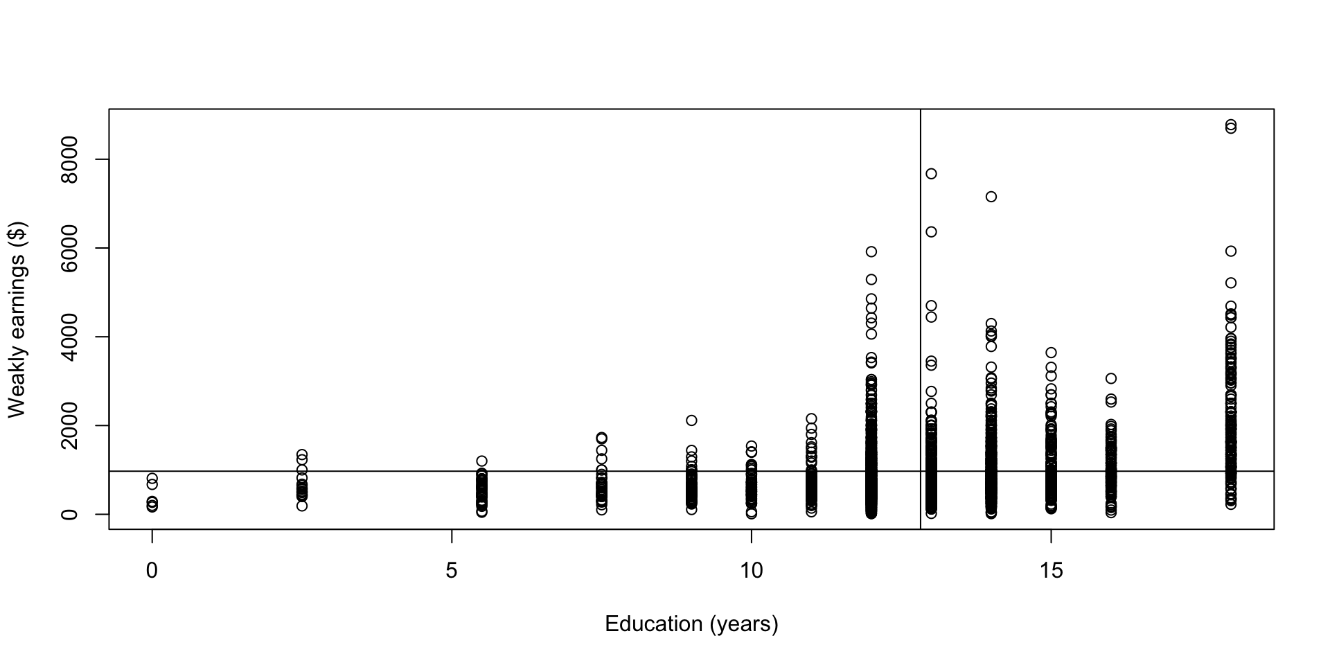
This doesn’t necessarily mean higher education caused more earnings. There are many other factors affecting earnings, you name it.
Caveat for sample correlation
Correlation is not causation
Causal inference require more rigorous research design, such as randomized control trials, or more other methods that use observational data which you’ll learn more in more advanced course such as econometrics.
Linear transformation
Suppose \(v\) and \(w\) are linear transformations of \(x\) and \(y\) such that \(v=a+bx\) and \(w=c+dy\)
The sample covariance and correlation of \(v,w\) has the following relationship to the sample covariance and correlation of \(x,y\):
- Sample covariance: \[s_{vw}=bds_{cy}.\]
- Sample correlation: \[r_{vw}=\frac{bd}{|b||d|}r_{xy}.\]
You don’t need to memorize this, proof on JA pp. 190
Linear combinations of two variables
Suppose \(v\) is a linear combinations of \(x\) and \(y\) such that \(v=k+ax+by\)
The descriptive statistics of \(v\) hase the following relationship to the descriptive statistics of \(x,y\):
- Sample mean: \[\overline{v}=k+a\overline{x}+b\overline{y}\]
- Sample variance: \[s_v^2=a^2s_x^2+b^2s_x^2+2abs_{xy}\]
- Sample standard deviation: \[s_v=\sqrt{s_v^2}\]
Unfortunately the proof is omitted in JA text, but we’ll use simulation to show it in our lab session
Thanks! I’ll take any questions about HW or exam prep

ECON2250 Statistics for Economics - Fall 2025 - Maghfira Ramadhani