Simple Linear Regression

Week 13

Maghfira Ramadhani

Nov 12, 2025

Plan

1. Motivation: correlation, causality, and prediction
   
2. Model: \(Y = \alpha + \beta X + U\)
   
3. Least-Squares Estimator (LSE)
   
4. Geometric intuition of OLS
   
5. Empirical example (cigarette data)
   
6. Prediction vs causality
   
7. Check Your Understanding & Exit Question

Textbook Reference: JA Chapter 17

Motivation

• Correlation tells us how two variables move together.
  
• Regression quantifies how much \(Y\) changes when \(X\) changes.
  
• Two perspectives:
  • Predictive: best line for forecasting \(Y\) from \(X\)
    
  • Causal: effect of changing \(X\) on \(Y\)

The Model

\[ Y_i = \alpha + \beta X_i + U_i \]

where

• \(Y_i\): dependent (response) variable
  
• \(X_i\): independent (explanatory) variable
  
• \(\alpha\): intercept
  
• \(\beta\): slope (effect of \(X\) on \(Y\))
  
• \(U_i\): unobserved factors

Assumption: \(E[U_i|X_i] = 0\) ensures unbiased estimation.

Least Squares Estimator (LSE)

Goal: minimize the Sum of Squared Residuals

\[ S(\alpha,\beta)=\sum_i (Y_i - \alpha - \beta X_i)^2 \]

First-order conditions:

\[ \frac{\partial S}{\partial \alpha}=0,\quad \frac{\partial S}{\partial \beta}=0 \]

Solution:

\[ \hat{\beta}=\frac{\sum_i (X_i-\bar{X})(Y_i-\bar{Y})}{\sum_i (X_i-\bar{X})^2},\qquad \hat{\alpha}=\bar{Y}-\hat{\beta}\bar{X}. \]

R Example: Computing LSE Manually

data(cigdata)

x <- cigdata$cigtax
y <- cigdata$cigsales

beta_hat  <- cov(x, y) / var(x)
alpha_hat <- mean(y) - beta_hat * mean(x)
c(alpha_hat, beta_hat)

[1] 55.948902 -9.487131

Using lm() in R

model <- lm(cigsales ~ cigtax, data = cigdata)
summary(model)

Call:
lm(formula = cigsales ~ cigtax, data = cigdata)

Residuals:
    Min      1Q  Median      3Q     Max 
-23.921  -8.098  -0.857   5.014  39.338 

Coefficients:
            Estimate Std. Error t value Pr(>|t|)    
(Intercept)   55.949      3.244  17.249  < 2e-16 ***
cigtax        -9.487      1.511  -6.277 8.75e-08 ***
---
Signif. codes:  0 '***' 0.001 '**' 0.01 '*' 0.05 '.' 0.1 ' ' 1

Residual standard error: 12.52 on 49 degrees of freedom
Multiple R-squared:  0.4457,    Adjusted R-squared:  0.4344 
F-statistic:  39.4 on 1 and 49 DF,  p-value: 8.754e-08

Interpretation:
- Intercept (\(\hat{\alpha}\)) – predicted sales if tax = 0
- Slope (\(\hat{\beta}\)) – change in sales per $1 increase in tax

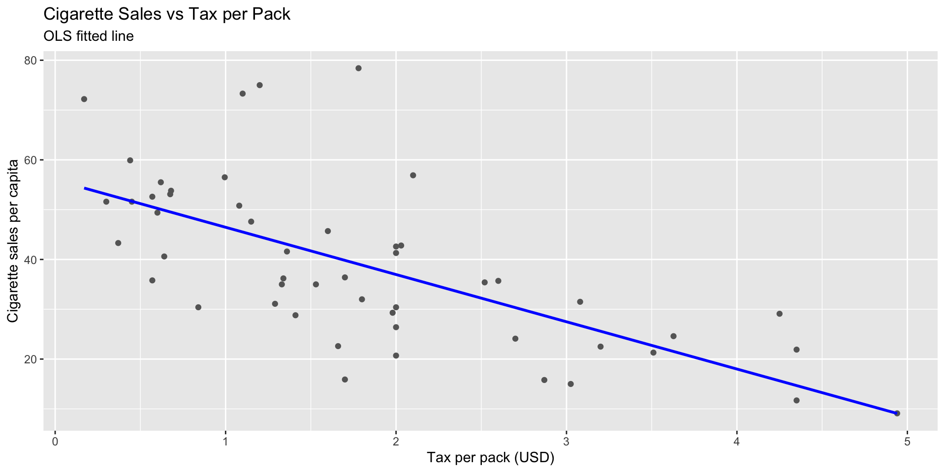
Visualizing the Regression Line

ggplot(cigdata, aes(x=cigtax, y=cigsales)) +
  geom_point(color="grey40") +
  geom_smooth(method="lm", se=FALSE, color="blue") +
  labs(title="Cigarette Sales vs Tax per Pack",
       subtitle="OLS fitted line",
       x="Tax per pack (USD)", y="Cigarette sales per capita")

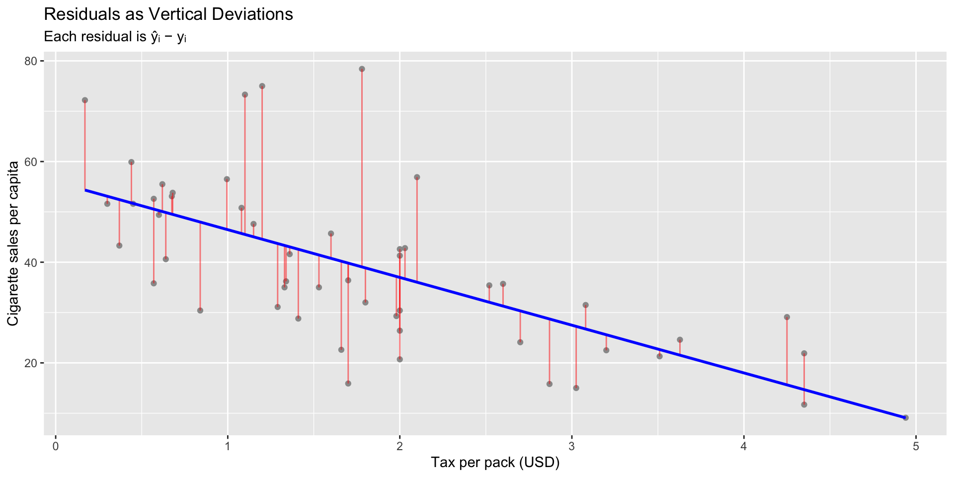
Residuals and Fit Illustration

cigdata <- cigdata |>
  mutate(fitted = fitted(model),
         resid  = resid(model))

ggplot(cigdata, aes(x=cigtax, y=cigsales)) +
  geom_point(color="grey60") +
  geom_segment(aes(xend=cigtax, yend=fitted), color="red", alpha=0.5) +
  geom_smooth(method="lm", se=FALSE, color="blue") +
  labs(title="Residuals as Vertical Deviations",
       subtitle="Each residual is ŷᵢ − yᵢ",
       x="Tax per pack (USD)", y="Cigarette sales per capita")

Geometry of OLS

• The regression line minimizes the distance (in squared sense) from all points to the line.
  
• Residuals are orthogonal to fitted values:

\[ \sum_i \hat{u}_i = 0,\quad \sum_i X_i \hat{u}_i = 0. \]

Economic Interpretation

• \(\beta\) measures marginal effect: how much \(Y\) changes for one-unit change in \(X\).
  
• Sign of \(\beta\) follows sign of correlation \(r_{XY}\).
  
• \(\alpha\) gives baseline level when \(X=0\).
  
• Units matter for interpretation.

Prediction vs Causality

Prediction	Causality
Goal: minimize prediction error	Goal: estimate causal effect
Focus on fit \(E[Y|X]\)	Requires \(E[U|X]=0\)
Works with any \(X\)–\(Y\) relation	Needs exogenous variation
“What \(Y\) do I expect if \(X = x\)?”	“What happens to Y if I change X?”

Inference for the Slope Parameter

When assumptions hold:

\[ t = \frac{\hat{\beta} - \beta_0}{se(\hat{\beta})} \quad \sim \; t_{n-2}. \]

Use summary(model) in R to see \(t\) statistic and p-value.

Check Your Understanding

1. Using the regression of cigsales on cigtax, interpret the slope’s sign and magnitude.
   
2. If the tax increased by $0.50, what is the predicted change in sales?
   
3. Does this relationship necessarily mean higher taxes cause lower sales? Why or why not?

Exit Question

Under what condition can the regression coefficient \(\beta\) be interpreted as a causal effect?

Only if the exogeneity condition \(E[U|X]=0\) holds — that is, when changes in \(X\) are not systematically related to the unobserved factors \(U\).