Estimation and Confidence Intervals
Week 10
Plan
In today’s lecture, we will learn about:
- Estimator and its desired properties
- Confidence intervals of sample mean of normal random variables (finite sample)
- One-sided confidence intervals
- Two-sided confidence intervals
- Confidence intervals of sample mean from large sample
Textbook Reference: JA 14
Estimator
| Estimand \(\theta\) | Estimator \(\hat{\theta}_X\) | Estimate \(\hat{\theta}_X\) | |
|---|---|---|---|
| Mean | \(\mu_X\) | \(\bar{X}\) | \(\bar{x}\) |
| Variance | \(\sigma_X^2\) | \(s_X^2\) | \(s_x^2\) |
| Standard Deviation | \(\sigma_X\) | \(s_X\) | \(s_x\) |
| Median | \(\tau_{X,0.5}\) | \(\tilde{X}_{0.5}\) | \(\tilde{x}_{0.5}\) |
| Median | \(\tau_{X,q}\) | \(\tilde{X}_{q}\) | \(\tilde{x}_{q}\) |
| IQR | \(\tau_{X,0.75}-\tau_{X,0.25}\) | \(\tilde{x}_{0.75}-\tilde{x}_{0.25}\) | \(\tilde{x}_{0.75}-\tilde{x}_{0.25}\) |
| Correlation | \(\rho_{XY}\) | \(r_{XY}\) | \(r_{xy}\) |
- Estimand = parameter or quantity of interests
- Estimator = a random variable before we observe our sample
- Estimate = realization of estimator after sample is observed or the calculated statistics
Property of estimator
Unbiased: \(E(\hat{\theta}_X)=\theta\) for any sample size \(n\)
Consistent: \(\hat{\theta}_X\underset{p}{\rightarrow} \theta \quad \text{ as } n\rightarrow\infty.\)
Asymptotically normal: \(\hat{\theta}_X\overset{p}{\sim} N(\theta,\frac{V}{n}) \quad \text{ as } n\rightarrow\infty.\)
Efficiency: An estimator is more efficient when the asymptotic variance is smaller.
We’ve discussed some example of estimator:
Sample mean \(\bar{X}=\frac{1}{n}\sum_i X_i\) is unbiased estimator of population mean \(\mu_X=E(X)\)
Sample variance \(s_X^2=\frac{1}{n-1}\sum_i (X_i-\bar{X})^2\) is unbiased estimator of population variance \(\sigma_X=Var(X)=E((X-\mu_X)^2)\)
Confidence intervals
Confidence intervals: an interval of plausible values for a parameter/estimands \(\theta\) based on an estimator \(\hat{\theta}_X\).
A 95% confidence interval for the for a parameter is an interval for which, before observing the sample, there is 95% probability that the parameter is in the interval created by the estimation procedure
Confidence intervals: Normal
Assume \(X_i\overset{iid}{\sim} N(\mu,\sigma^2)\)
Goal: Estimate the confidence interval for \(\mu\) based on the sample mean estimator \(\bar{X}\)
We start from results from previous class: \[\bar{X}\overset{a}{\sim} N\left(\mu,\frac{\sigma^2}{n}\right)\quad\text{ or }\quad \frac{\bar{X}-\mu}{\sigma/\sqrt{n}}\overset{a}{\sim} N\left(0,1\right).\]
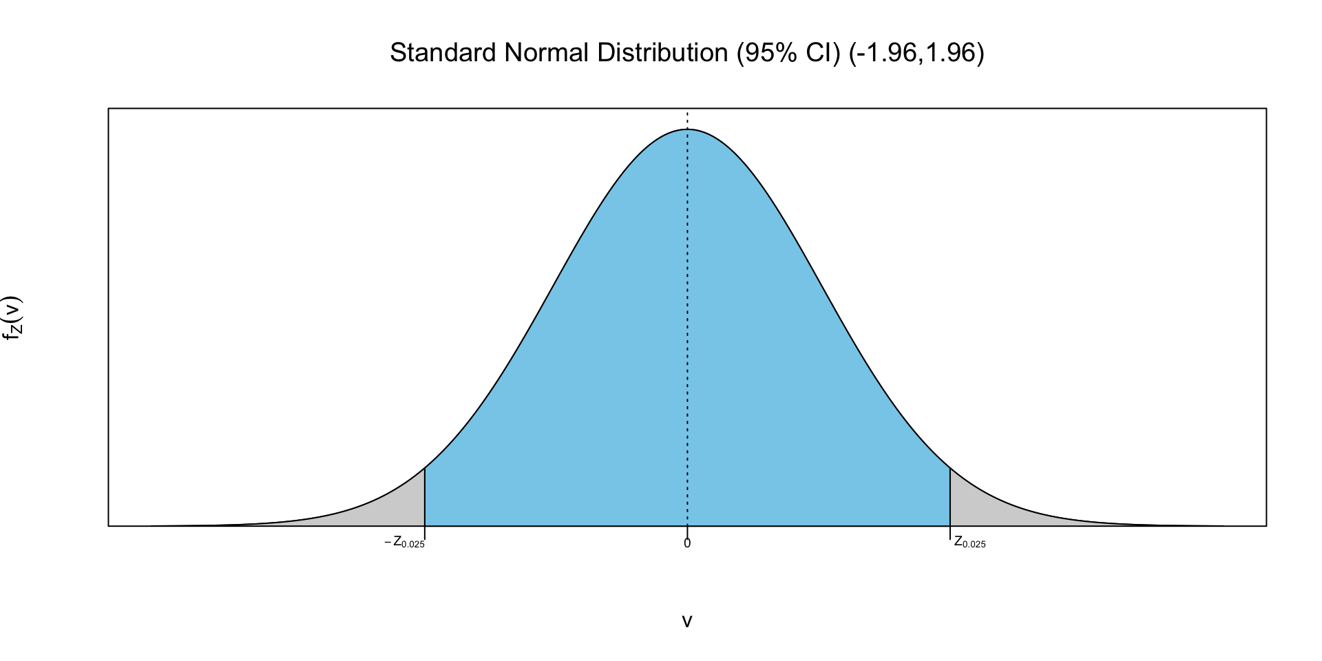
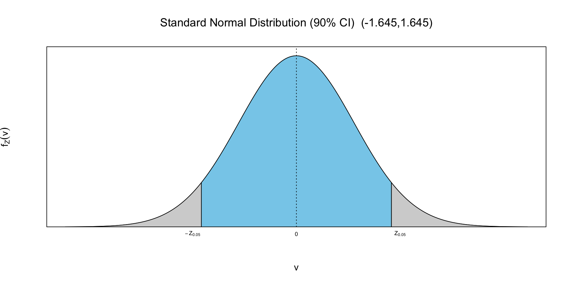
Assuming we know \(\mu\) and \(\sigma\), then the 95% probability interval for \(\bar{X}\) is \[\left(\mu-1.96\frac{\sigma}{\sqrt{n}},\mu+1.96\frac{\sigma}{\sqrt{n}}\right)\] where -1.96 is the 2.5% quantile of standard normal and 1.96 is the 97.5% quantile of standard normal.
Confidence intervals: Normal
Confidence intervals: Normal
Confidence intervals: Normal
We want to play around a little bit so that we got the confidence interval for \(\mu\)
The 95% probability interval for \(\mu\) is \[P\left(\bar{X}-1.96\frac{\sigma}{\sqrt{n}}< \mu<\bar{X}+1.96\frac{\sigma}{\sqrt{n}}\right)=0.95\] where -1.96 is the 2.5% quantile of standard normal and 1.96 is the 97.5% quantile of standard normal.
Replacing the estimator with our estimate, the 95% confidence interval for \(\mu\) is \[P\left(\bar{x}-1.96\frac{\sigma}{\sqrt{n}}< \mu<\bar{x}+1.96\frac{\sigma}{\sqrt{n}}\right)=0.95\] where -1.96 is the 2.5% quantile of standard normal and 1.96 is the 97.5% quantile of standard normal.
Can we use this directly? We know \(n\) but do we know \(\sigma\)?
Confidence intervals: Normal, Unknown Variance
What if we use estimator for \(\sigma\), i.e., our sample standard deviation \(s_X\)?
Go back to previous class \[\frac{\bar{X}-\mu}{\sigma/\sqrt{n}}\overset{a}{\sim} N\left(0,1\right)\quad \text{ but }\quad\frac{\bar{X}-\mu}{s_X/\sqrt{n}}\overset{}{\sim} \text{?}\]
We know that \(\bar{X}-\mu\) is normal, but what is the distribution of \(s_X\)?
Recall \(s_X^2=\frac{1}{n-1}\sum_i (X_i-\bar{X})^2\), what is the distribution of the sum of normal?
Confidence intervals: Normal, Unknown Variance
Turns out when we have two random variables \(Y\) and \(Z\) such that \(Y\sim\chi_m^2\) and \(Z\sim N(0,1)\), then a random variable \[W=\frac{Z}{\sqrt{Y/m}}\sim t_m\] where \(t_m\) is \(t\)-distribution with \(m\) degree of freedom
With some math (omitted), if we assume \(X_i\overset{iid}{\sim} N(\mu,\sigma^2)\) then \[\frac{\bar{X}-\mu}{s_X/\sqrt{n}}\overset{}{\sim}t_{n-1}\]
Confidence intervals: Normal, Unknown Variance
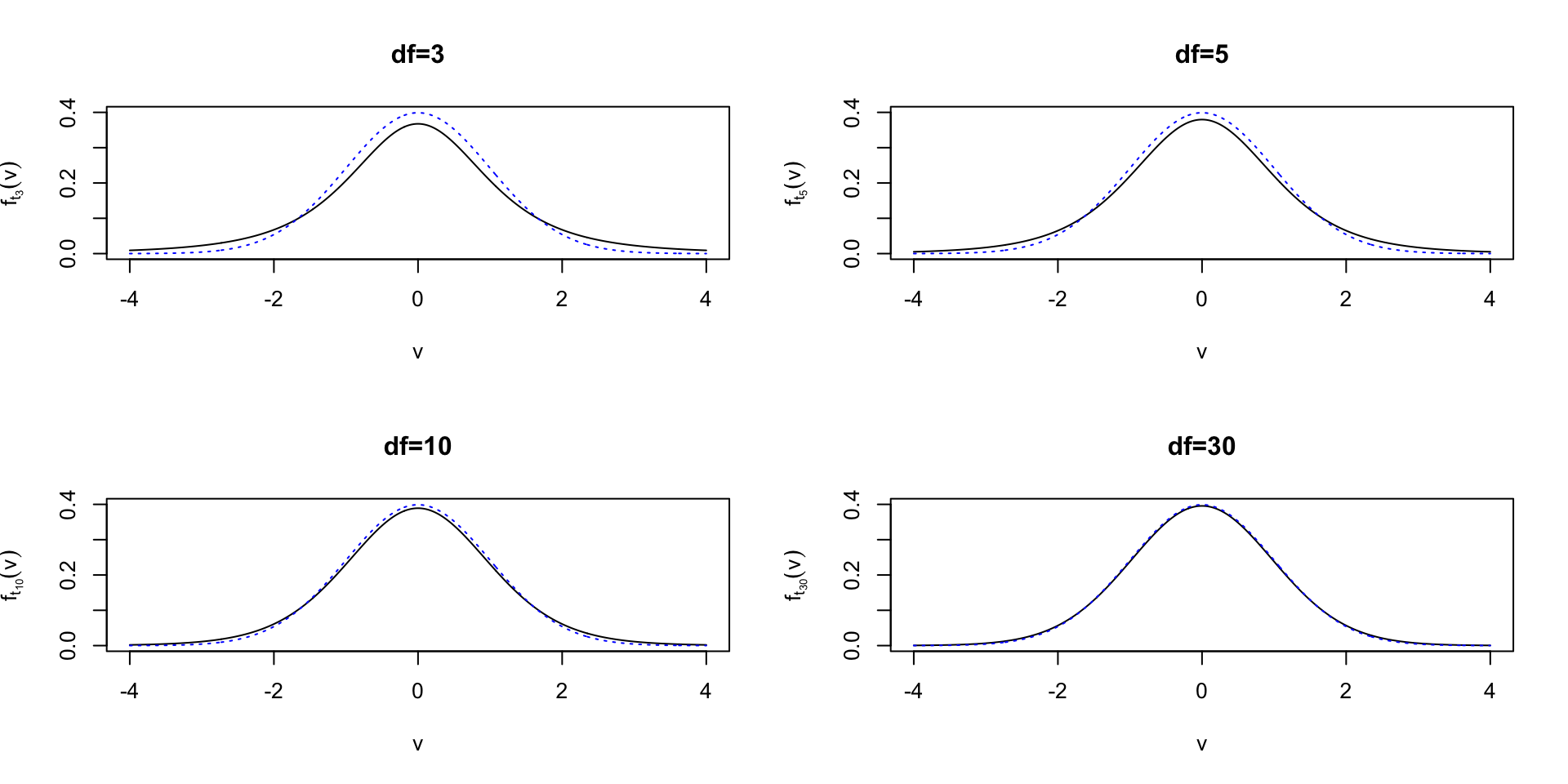
t-distribution approximate normal for large \(n\)
Confidence intervals: Normal, Unknown Variance
t-distribution approximate normal for large \(n\)
Confidence intervals: Normal, Unknown Variance
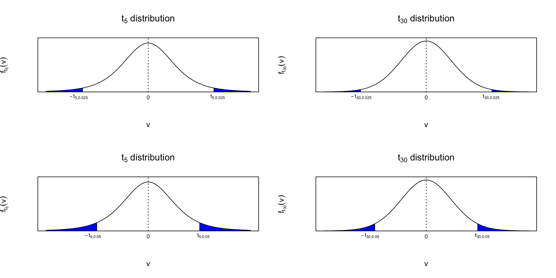
- The 95% probability interval for \(\bar{X}\) is \[P\left(\bar{X}-t_{n-1,0.025}\frac{s_X}{\sqrt{n}}< \mu<\bar{X}+t_{n-1,0.025}\frac{s_X}{\sqrt{n}}\right)=0.95\] where \(t_{n-1,0.025}\) is the quantile of \(t\)-distribution with \(n-1\) degree of freedom at 97.5% (1-0.025)
Confidence intervals: Normal, Unknown Variance
Now we can use our estimator to get the confidence intervals.
The 95% confidence interval for \(\mu\) is \[P\left(\bar{x}-t_{n-1,0.025}\frac{s_x}{\sqrt{n}}< \mu<\bar{x}+t_{n-1,0.025}\frac{s_x}{\sqrt{n}}\right)=0.95\] where \(t_{n-1,0.025}\) is the quantile of \(t\)-distribution with \(n-1\) degree of freedom at 97.5% (1-0.025)
More generalized version, the (1-\(\alpha\)) confidence interval for \(\mu\) is \[P\left(\bar{x}-t_{n-1,\alpha/2}\frac{s_x}{\sqrt{n}}< \mu<\bar{x}+t_{n-1,\alpha/2}\frac{s_x}{\sqrt{n}}\right)=1-\alpha\] where \(t_{n-1,\alpha/2}\) (a.k.a. critical value) is the quantile of \(t\)-distribution with \(n-1\) degree of freedom at (1-\(\alpha/2\))
Confidence intervals: Example
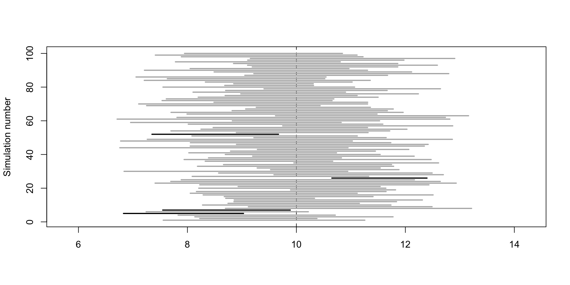
Confidence intervals: Intuition
Simulation of random sample of n=8 from \(N(10,4)\)
Confidence intervals: One sided
What if we’re interested in one-sided confidence interval for \(\mu\)?
Using the same method as before, we can get the probability interval for \(\mu\): \[P\left(\mu>\bar{X}-t_{n-1,\alpha}\frac{s_X}{\sqrt{n}}\right)=1-\alpha\] and similarly \[P\left(\mu<\bar{X}+t_{n-1,\alpha}\frac{s_X}{\sqrt{n}}\right)=1-\alpha\]
Confidence intervals: One sided
- The associated \(1-\alpha\) confidence interval for \(\mu\) is given by \[\left(\bar{x}-t_{n-1,\alpha}\frac{s_x}{\sqrt{n}},\infty\right)\] and similarly \[\left(-\infty,\bar{x}+t_{n-1,\alpha}\frac{s_x}{\sqrt{n}}\right)\]
Confidence intervals: Large \(n\)
- Leveraging the asymptotically normal distirbution of large sample size, we can use normal quantile instead of t-distribution quantiles.
- Two-sided confidence interval for \(\mu\): the (1-\(\alpha\)) confidence interval for \(\mu\) is \[P\left(\bar{x}-z_{\alpha/2}\frac{s_x}{\sqrt{n}}< \mu<\bar{x}+z_{\alpha/2}\frac{s_x}{\sqrt{n}}\right)=1-\alpha\] where \(z_{\alpha/2}\) is the \(1-\alpha/2\) quantile of standard normal
- One-sided confidence interval for \(\mu\): the \(1-\alpha\) confidence interval for \(\mu\) is given by \[\left(\bar{x}-t_{n-1,\alpha}\frac{s_x}{\sqrt{n}},\infty\right)\quad\text{and}\quad\left(-\infty,\bar{x}+t_{n-1,\alpha}\frac{s_x}{\sqrt{n}}\right)\]
Confidence intervals: Example
Up next
- Research topics due tonight
- HW4 assigned tomorrow
- Hypothesis testing next week