Expectation and Moments

Week 9

Maghfira Ramadhani

Oct 13, 2025

Plan

In today’s lecture, we will learn about:

1. Expectation of a random variable
   
2. Properties of expectation
   
3. Variance and standard deviation
   
4. Moments and their relation to mean and median
   
5. Covariance and correlation
   
6. Conditional expectation

Textbook Reference: SDG 4.1–4.7

Concepts

Concept	Definition	Interpretation
\(E[X]\)	Mean	Long-run average
\(Var(X)\)	Variance	Spread around mean
\(Cov(X,Y)\)	Covariance	Joint variability
\(\rho_{XY}\)	Correlation	Strength of linear relationship
\(E[Y|X]\)	Conditional expectation	Best prediction of \(Y\) given \(X\)

Expectation of a Random Variable

Expectation (or the population mean) of a random variable summarizes its central tendency.

• For a discrete r.v. \(X\) with pmf \(p_X(x)\): \[E[X] = \sum_x x p_X(x)\]

• For a continuous r.v. \(X\) with pdf \(f_X(x)\): \[E[X] = \int_{-\infty}^{\infty} x f_X(x) dx\]

Intuition: The expectation is the long-run average value if we repeatedly observe \(X\).

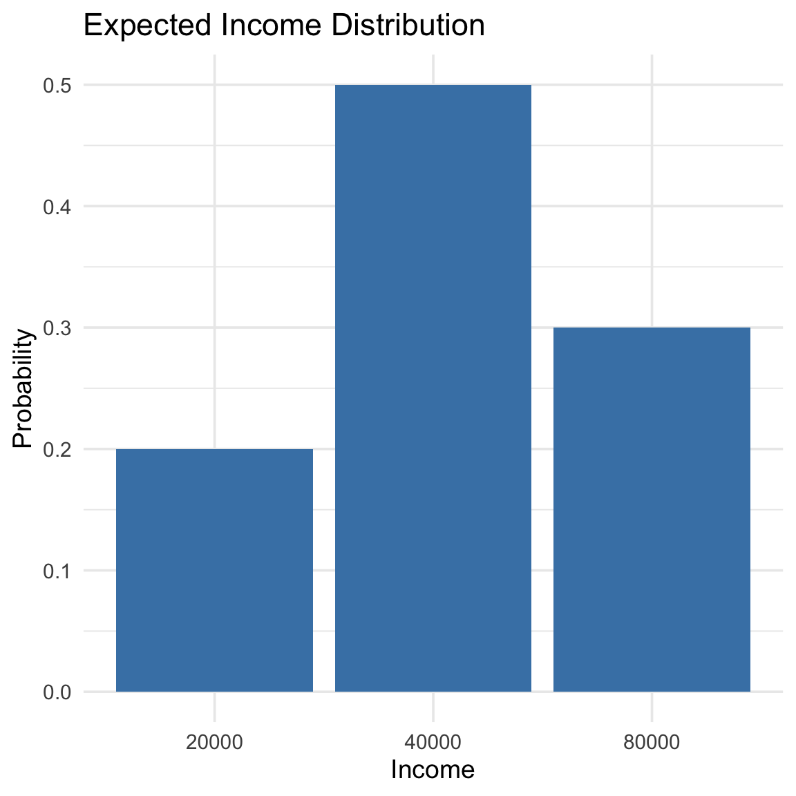
Example: Expected income

Income (\(x\))	Probability \(p(x)\)
20,000	0.2
40,000	0.5
80,000	0.3

\[E[X] = 20{,}000(0.2) \\+ 40{,}000(0.5) \\+ 80{,}000(0.3) \\= 48{,}000.\]

Properties of Expectation

Let \(a,b\) be constants and \(X,Y\) random variables.

1. Linearity:
   \[E[aX + b] = aE[X] + b\]
2. Additivity:
   \[E[X+Y] = E[X] + E[Y]\]
3. Independence:
   If \(X\) and \(Y\) are independent, \(E[XY] = E[X]E[Y]\).

Application Example

A survey records the number of streaming subscriptions in 3 independent households. Let \(S_i\) be the subscriptions in household \(i\), where \(i \in \{1, 2, 3\}\). Each household has the following probability mass function (pmf): \[ P(S_i=0)=0.5,\quad P(S_i=1)=0.3,\quad P(S_i=2)=0.2. \] Let \(X = S_1 + S_2 + S_3\) be the total subscriptions across 3 independent households.

Since \(S_1,S_2,S_3\) are independent and identically distributed (i.i.d) following the given pmf, we have \[E(X)=E(S_1+S_2+S_3)=E(S_1)+E(S_2)+E(S_3)=3E(S_i).\]

Using the given pmf we can compute \(E(S_i)=\sum_{j}s_j P(S_i=s_j).\)

Variance

Variance measures the dispersion of a random variable around its mean.

\[Var(X) = E[(X - E[X])^2] = E[X^2] - (E[X])^2.\]

The standard deviation is: \[\sigma_X = \sqrt{Var(X)}.\]

Variance as Expected Squared Deviation

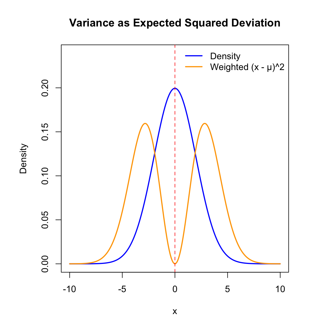
• Variance captures the expected squared distance from the mean.
  
• The orange curve shows how \((x - \mu)^2\) is weighted by the probability density.
  
• Most of the contribution to \(Var(X)\) comes from values close to the mean.
  

Property of Variance

Let \(a,b\) be constants and \(X,Y\) random variables.

1. Linear function:
   Let \(Y=aX+b\) then \[Var(Y)=Var(aX + b) = a^2Var(X)\]
2. Sum of independent random variable:
   If \(X\) and \(Y\) are independent, \(Var(X+Y) = Var(X)+Var(Y)\).

Moments

For random variable \(X\) and positive integer \(k\), \(E(X^k)\) is called the \(k\)-th moment of \(X\).

Moments provide additional information about the shape of a distribution.

• The first moment about zero: \(E[X]\)
• The second moment about zero: \(E[X^2]\)
• The second moment about the mean is the variance.

Higher moments describe: - Skewness (asymmetry) - Kurtosis (tailedness)

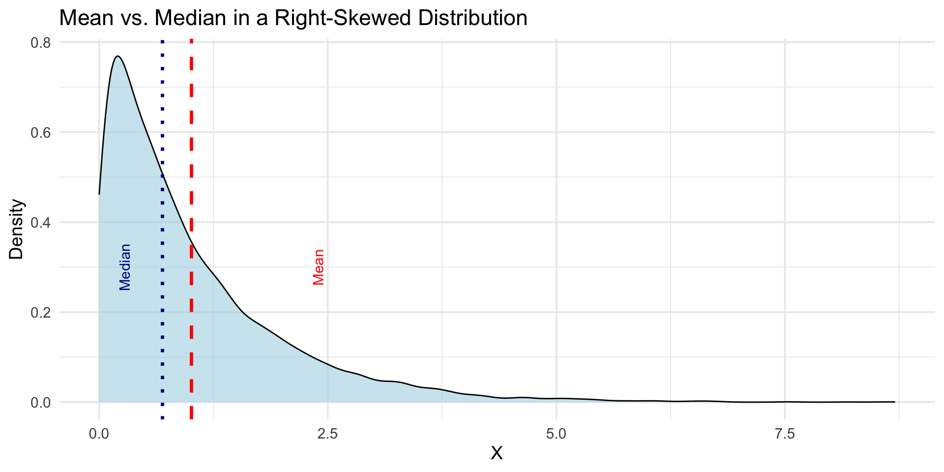
The Mean and the Median

• The mean minimizes squared deviations:
  \[E[(X - a)^2]\] is minimized when \(a = E[X].\)
• The median minimizes absolute deviations:
  \[E[|X - a|]\] is minimized when \(a\) is the median.

For those interested, proof available on SDG pp244-245

The Mean and the Median

Covariance and Correlation

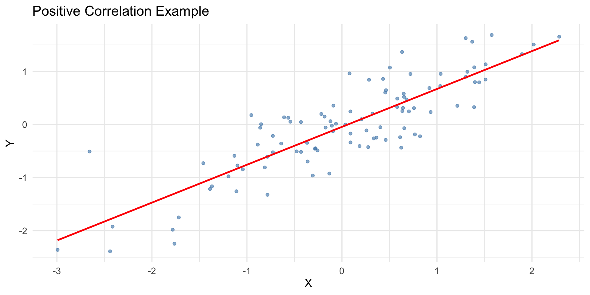
Covariance measures joint variability between two variables: \[Cov(X,Y) = E[(X - E[X])(Y - E[Y])]=E[XY]-E[X]E[Y].\]

Correlation standardizes covariance: \[\rho_{XY} = \frac{Cov(X,Y)}{\sigma_X \sigma_Y}.\]

Property of Covariance and Correlation

Let \(a,b\) be constants and \(X,Y\) random variables.

1. Independence:
   If \(X\) and \(Y\) are independent, \(Cov(X,Y) = \rho(X,Y)=0\).
2. Linear function:
   Let \(Y=aX+b\) where \(a\neq 0\) then \[\rho(X,Y)=\begin{cases}1 &\text{ if }a>0,\\-1 &\text{ if }a<0.\end{cases}\]
3. Sum of two random variable:
   \(Var(X+Y) = Var(X)+Var(Y)+Cov(X,Y)\).

Visual Example

Conditional Expectation

Conditional expectation is the expected value of \(Y\) given information about \(X\).

\[E[Y|X=x] = \sum_y y \, p_{Y|X}(y|x) \quad \text{or} \quad \int y f_{Y|X}(y|x) dy.\]

It represents the best predictor of \(Y\) given \(X\).

In other words, predictor \(d(X)=E[Y|X]\) minimize the mean squared error (MSE) or \(E[(Y-d(X))^2]\).

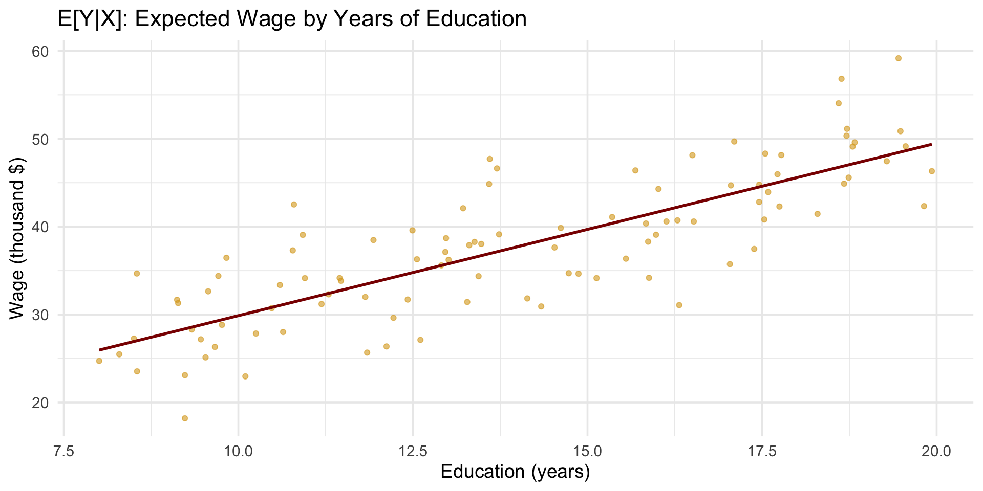
Example: Wage and Education

Let \(Y\) be wage and \(X\) be years of education.

• \(E[Y|X=x]\) gives the expected wage for a person with \(x\) years of education.
  
• The conditional expectation curve \(E[Y|X]\) is the regression function.

Wrap-Up

Concept	Definition	Interpretation
\(E[X]\)	Mean	Long-run average
\(Var(X)\)	Variance	Spread around mean
\(Cov(X,Y)\)	Covariance	Joint variability
\(\rho_{XY}\)	Correlation	Strength of linear relationship
\(E[Y|X]\)	Conditional expectation	Best prediction of \(Y\) given \(X\)

Summary

• Expectation summarizes the “center” of a distribution.
  
• Variance, covariance, and correlation describe variability and relationships.
  
• Mean and median differ in skewed data.
  
• Conditional expectation forms the foundation of regression analysis.

Next lecture: Exam II Review

Fill out this form please