Model of Continuous Random Variables
Week 8
Oct 08, 2025
Plan
In today’s class we will learn commonly used models for continuous random variables:
- Normal random variables
- Log-normal random variables
- Chi-square random variables
- Exponential random variables
Textbook Reference: JA 11; SDG 5.6, 8.2
Continuous random variables
- Discrete r.v.: take on countable set of values (0,1,2,…).
- Continuous r.v.: can take on any value in an interval.
- Described by a probability density function (pdf) \(f(x)\) such that:
\[
P(a \leq X \leq b) = \int_a^b f(x) dx
\]
- \(f(x)\ge 0\) for all \(x\), and \(\int_{-\infty}^{\infty} f(x) dx = 1\).
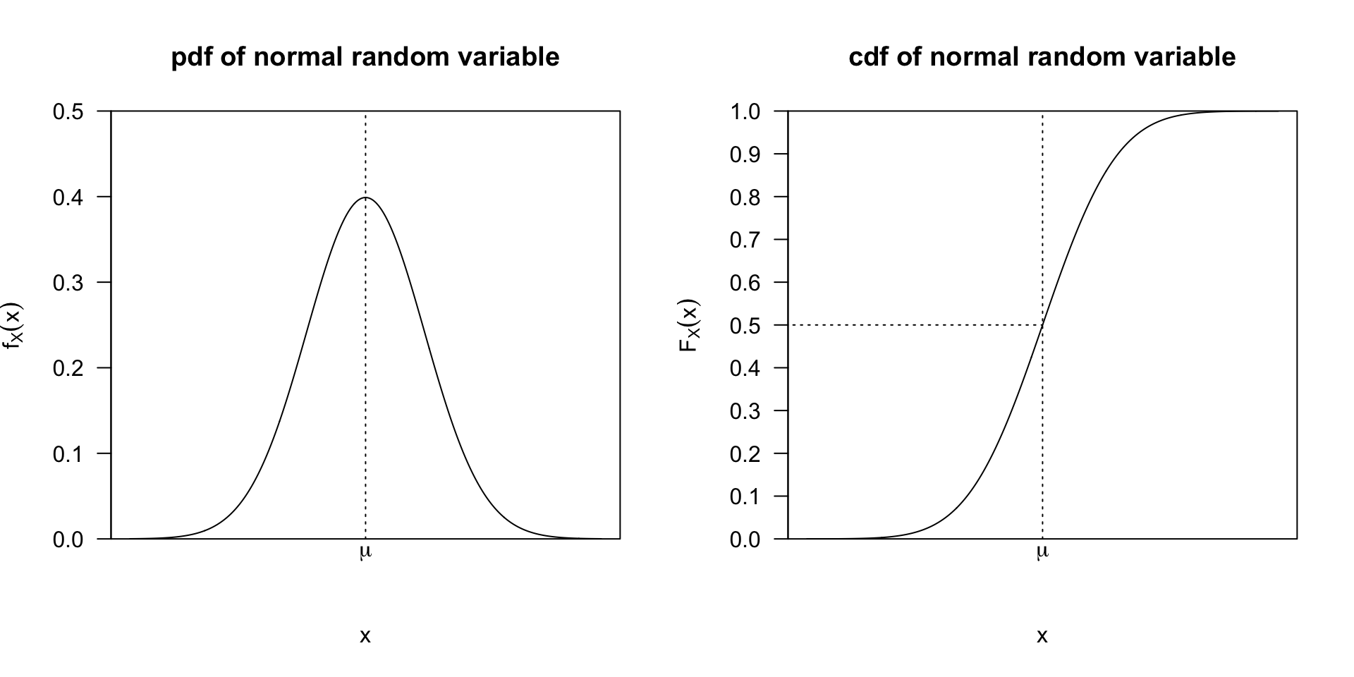
Normal random variables
A random variable \(X\) has a normal distribution with mean \(\mu\) and variance \(\sigma^2\), written \(X\sim N(\mu,\sigma^2)\), if its pdf is
\[
f_X(x|\mu,\sigma^2) = \frac{1}{\sqrt{2\pi\sigma^2}} \exp\left(-\frac{(x-\mu)^2}{2\sigma^2}\right).
\]
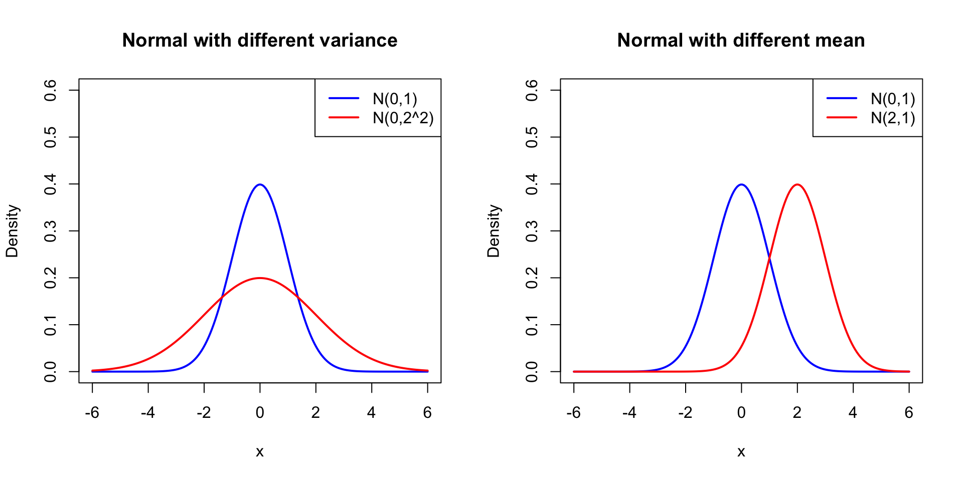
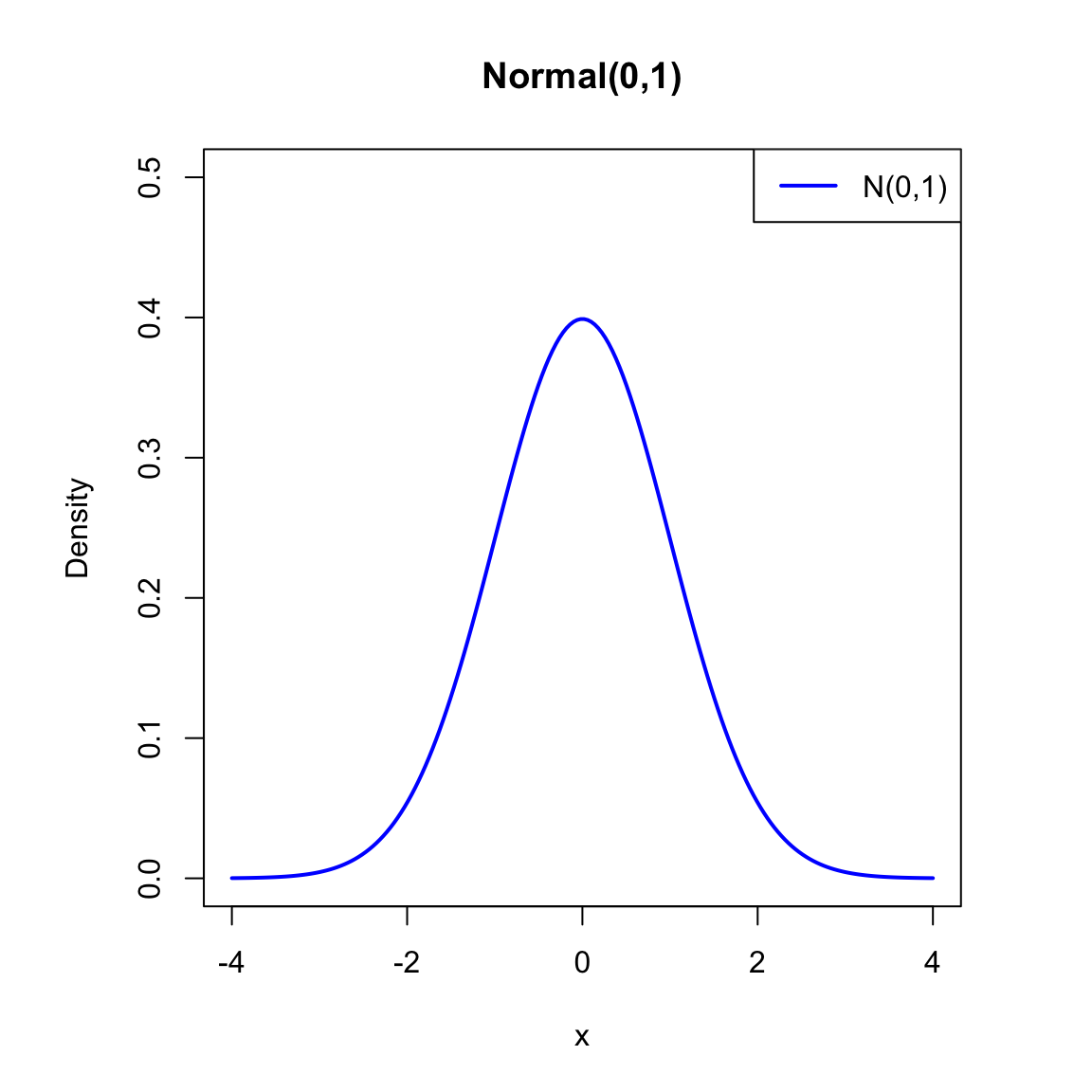
- Symmetric around \(\mu\), and has a bell-shaped curve.
- Parameters: mean (\(\mu\)) and variance (\(\sigma^2\)).
- Functions in R:
pnorm(x,mu,sd) # P(X <= x)
qnorm(p,mu,sd) # quantile at probability p
dnorm(x,mu,sd) # density at x
rnorm(n,mu,sd) # random draws
Normal random variables
![]()
Normal random variables
![]()
Normal random variables
![]()
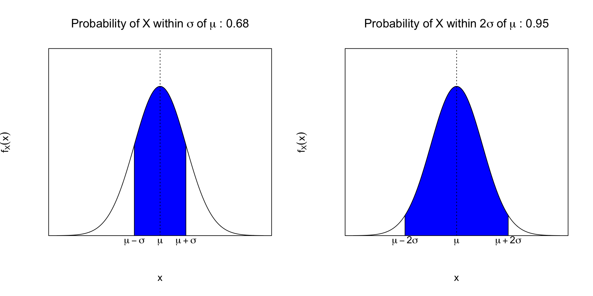
Standard normal
- If \(X\sim N(\mu,\sigma^2)\), then \(Z=\frac{X-\mu}{\sigma}\sim N(0,1)\).
- A standard normal pdf denoted \(\phi(z)\) and cdf denoted \(\Phi(z)\)
- Typically used in probability tables/software. \[P(-1.96\leq Z\leq 1.96)\approx 0.95\] \[P(-1.645\leq Z\leq 1.645)\approx 0.90\]
- Functions in R:
pnorm(z)     # P(Z <= z)
qnorm(p)     # quantile at probability p
dnorm(z)     # density at z
rnorm(n,mu,sd) # random draws
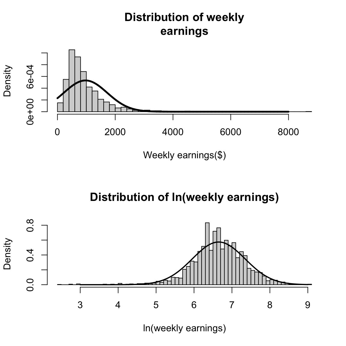
Log-normal random variables
If \(\ln X\sim N(\mu,\sigma^2)\),
then \(X\) is log-normal.
\(X\) only takes positive values.
Skewed right, long tail.
Useful in economics for modeling income, wealth, firm size
Functions in R:
plnorm(x,lnmu,lnsd) # P(X <= x)
qlnorm(p,lnmu,lnsd) # quantile at probability p
dlnorm(x,lnmu,lnsd) # density at x
rlnorm(n,lnmu,lnsd) # random draws
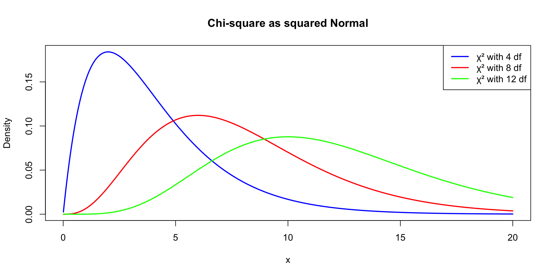
Chi-square
- If \(Z \sim N(0,1)\), then \(Z^2 \sim \chi^2_1\).
- More generally, if \(Z_1, Z_2, \ldots, Z_k \sim\) i.i.d. \(N(0,1)\), then
\[
X = Z_1^2 + Z_2^2 + \cdots + Z_k^2 \sim \chi^2_k
\]
- Key relationship: The chi-square distribution is built from the normal.
- Parameter \(k\) = degrees of freedom.
- Mean = \(k\), variance = \(2k\).
- Used in testing (goodness-of-fit, variance tests).
- Function in R:
pchisq(x,df), qchisq(p,df), dchisq(x,df), rchisq(n,df).
Chi-square
![]()
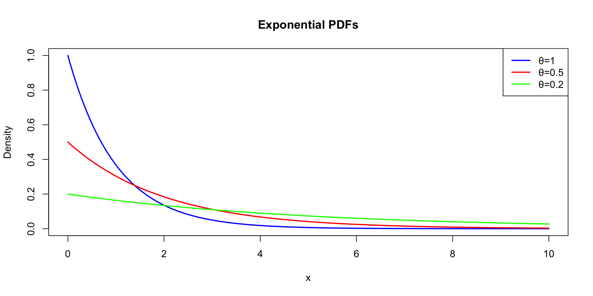
Exponential random variables
A random variable \(X\) is Exponential (\(\theta\)) if:
\[
f_X(x|\theta) = \theta e^{-\theta x},\quad x\ge 0
\]
- Mean = \(1/\theta\), variance = \(1/\theta^2\), CDF: \(F_X(x)=1-e^{-\theta x}.\)
- Applications:
- Duration of unemployment spells
- Time until a trade is executed
- Machine lifetimes
- Function in R:
pexp(x,rate), qexp(p,df), dexp(x,df), rexp(n,df).
Exponential random variables
![]()
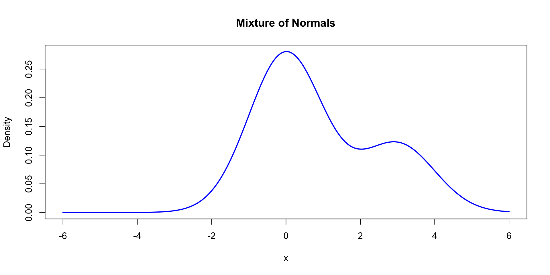
Mixtures of normals
- Some data look “normal-like” but with multiple peaks.
- A mixture of normals is a weighted average of normal distributions.
Economic example: distribution of daily sales may differ between weekdays and weekends.
![]()
Summary
We learned continuous random variable models:
- Normal: symmetric, bell-shaped, most common.
- Lognormal: positive, skewed, used for income/wealth.
- Chi-square: sums of squared normals, variance testing.
- Exponential: time durations, memoryless.
- Mixtures: flexible for multimodal data.