Lab 5: Simple Linear Regression
Week 14
Nov 17, 2025
Plan
In this lab we will practice:
- Visualizing linear relationships
- Estimating and interpreting simple linear regression models
- Computing slope and intercept manually and using R
- Evaluating model fit (R²) and residuals
- Reflecting on prediction vs. causality
Textbook Reference: JA Chapter 17
Warm-up & Review
Think about:
- What does the slope represent in a regression line?
- Does correlation imply causation?
- Why do we square residuals in OLS?
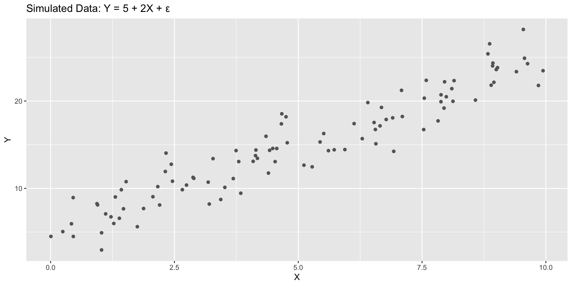
Exercise 1: Visualizing a Linear Relationship
Simulated data
Exercise 1: Visualizing a Linear Relationship
Task 1
Caution
- What sign do you expect for the correlation between
xandy?
- Add a fitted line using
geom_smooth(method="lm")and confirm visually.
Exercise 2: Manual OLS Estimation
Compute slope and intercept manually using formulas:
\[ \hat{\beta} = \frac{\sum_i (x_i - \bar{x})(y_i - \bar{y})}{\sum_i (x_i - \bar{x})^2}, \qquad \hat{\alpha} = \bar{y} - \hat{\beta}\bar{x}. \]
Exercise 2: Manual OLS Estimation
Compare with R’s built-in estimator:
Call:
lm(formula = y ~ x, data = simdata)

Residuals:
    Min      1Q  Median      3Q     Max
-4.4759 -1.2265 -0.0395  1.1927  4.4345

Coefficients:
            Estimate Std. Error t value Pr(>|t|)
(Intercept)  4.98208    0.39211   12.71   <2e-16 ***
x            1.98203    0.06836   28.99   <2e-16 ***
---
Signif. codes:  0 '***' 0.001 '**' 0.01 '*' 0.05 '.' 0.1 ' ' 1

Residual standard error: 1.939 on 98 degrees of freedom
Multiple R-squared:  0.8956,    Adjusted R-squared:  0.8945
F-statistic: 840.6 on 1 and 98 DF,  p-value: < 2.2e-16
Task 2
- Interpret the slope: what does a one-unit increase in \(X\) imply for \(Y\)?
- How close are your manual and R estimates? Why are they identical (up to rounding)?
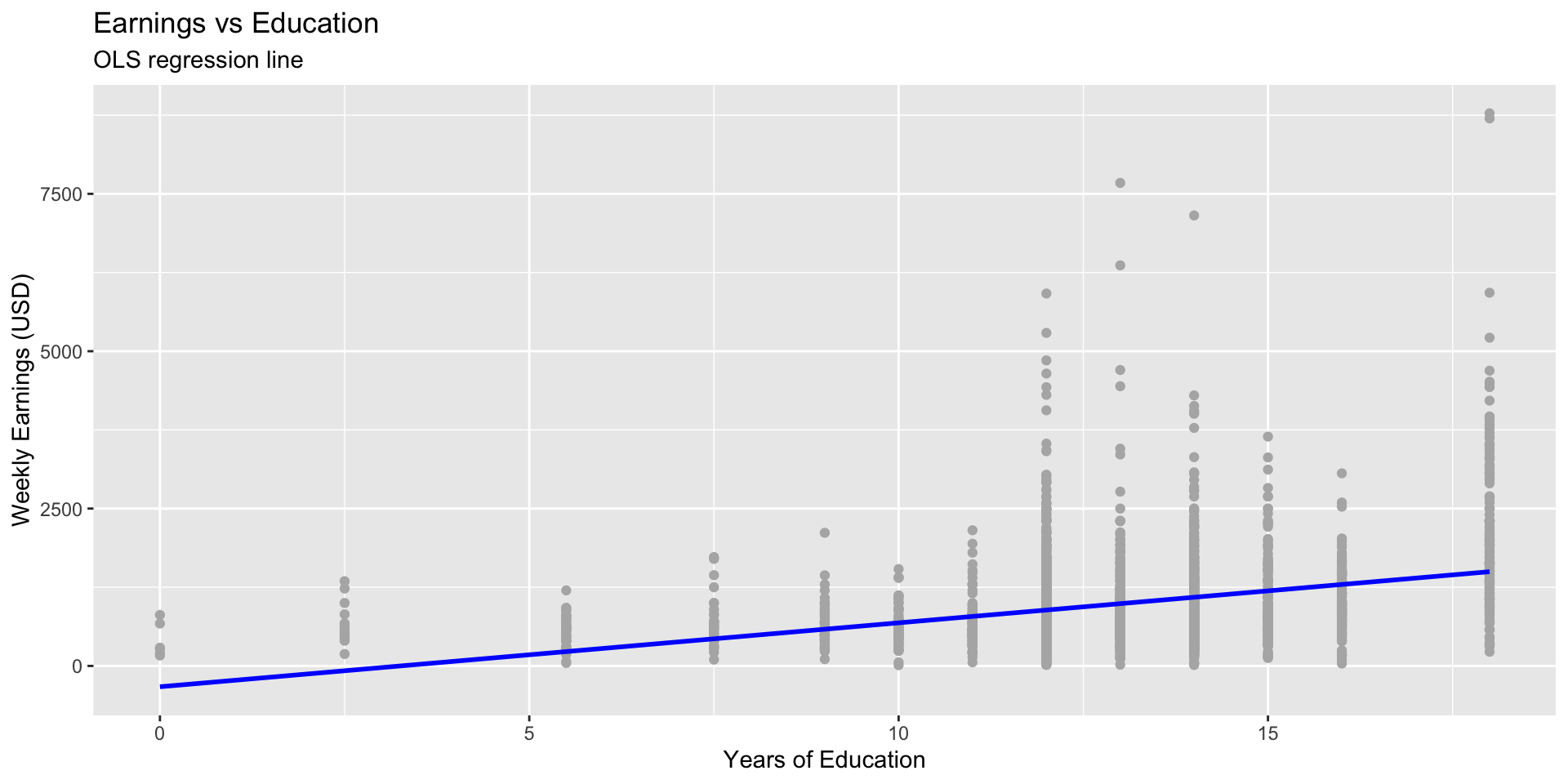
Exercise 3: Regression with CPS Data
Question: How does education relate to weekly earnings?
Call:
lm(formula = earnwk ~ educ, data = cps)

Residuals:
    Min      1Q  Median      3Q     Max
-1272.1  -417.3  -157.4   229.1  7282.6

Coefficients:
            Estimate Std. Error t value Pr(>|t|)
(Intercept) -330.753     72.713  -4.549 5.63e-06 ***
educ         101.550      5.575  18.217  < 2e-16 ***
---
Signif. codes:  0 '***' 0.001 '**' 0.01 '*' 0.05 '.' 0.1 ' ' 1

Residual standard error: 709.8 on 2807 degrees of freedom
  (1204 observations deleted due to missingness)
Multiple R-squared:  0.1057,    Adjusted R-squared:  0.1054
F-statistic: 331.9 on 1 and 2807 DF,  p-value: < 2.2e-16
Task 3
- Interpret the slope: how much does weekly earnings increase per year of education?
- Is the intercept meaningful here?
- Report \(R^2\) and explain what it measures.
Exercise 4: Visualizing the Fit
Task 4
- Add residual lines with
geom_segment().
- Identify one observation with a large positive and one with a large negative residual.
- What could explain them?
Exercise 5: Prediction and Causality
Use the fitted model to predict average earnings for 12, 14, and 16 years of education.
Task 5
- What happens to predicted earnings when education increases by 2 years?
- Can we interpret this as a causal effect of education on income? Why or why not?
- What omitted factors might bias the estimate?
Challenge Problem
Simulate a new dataset where \(Y = 5 + 2X + U\) but \(U\) is correlated with \(X\) (e.g., U <- 0.5*X + rnorm(n)).
Estimate the regression again and compare the slope.
Question: Does the estimated slope still recover the true value 2? Why not?
Exit Question
Under what condition can we interpret the slope \(\hat{\beta}\) as a causal effect?
Submission
Submit the rendered PDF or HTML report on Canvas as a group.
Be sure to include your plots, coefficient outputs, and short written interpretations.

ECON2250 Statistics for Economics – Fall 2025 – Maghfira Ramadhani