Lab 4: Hypothesis Testing

Week 12

Maghfira Ramadhani

Nov 03, 2025

Plan

In today’s lab, we will practice:

Conducting and interpreting one- and two-sample t-tests
Performing one- and two-sided tests manually and using built-in R functions
Simulating Type I error rates
Applying asymptotic (z) tests for large samples

Textbook Reference: JA Chapter 14 & 16
Lecture Slides: Hypothesis I, Hypothesis II

Quarto markdown file (.qmd) for today’s lab available on Canvas Module

Best Costume: Louvre Robbers #1 (Charlotte)

Thanks to other characters for participating:

Louvre Robbers #2, Lui*gi Mang*oni, Cat, Hotdogs, Lord Farquaad, Scientist, Hannah Montana, Wizard, Slytherin graduate, Santa Claus (CMIIW Levi??), Anime characters (Jaden).

Let me know if your characters is not mentioned.

Overview

Test Type	Statistic	Built-in Function	Manual Formula
Two-sided hypothesis	t-stat	`t.test(x, mu=c)`	$(\bar{x} - c) / (s_x / \sqrt{n})$
One-sided hypothesis	t-stat	`t.test(..., alternative="greater")`	Use one tail of t-distribution
Asymptotic (general)	z-stat	manual	$(\hat{\theta}-\theta_0)/se(\hat{\theta})$
Two-sample mean (Welch)	t-stat	`t.test(x, y, var.equal=FALSE)`	$(\bar{x}_1 - \bar{x}_2)/\sqrt{s_1^2/n_1 + s_2^2/n_2}$
Two-sample mean (Pooled)	t-stat	`t.test(x, y, var.equal=TRUE)`	$\sqrt{m+n-2}\dfrac{\bar{x}-\bar{y}}{\sqrt{1/m+1/n}\sqrt{s_x^2+s_y^2}}$
Correlation	z-stat	`cor.test()`	$(r - \rho_0)/\sqrt{(1-r^2)^2/n}$

Submission

Replicating and submitting pdf worth 70 points, each Task (Try and Reflect/Discuss) worth 5 points, Challenge Problem worth extra 5 points.
Change the name in the first page to your group member
Submit the rendered PDF by group on Canvas assignment by Monday 11:59 (Focus on presentation this week)

Warm-up & Review

Recall:

Null hypothesis ($H_0$) vs. Alternative hypothesis ($H_0$)
One-sided vs. Two-sided tests
Type I error ($\alpha$) and p-values

Warm-up:

In your own words, what does “reject $H_0$ at the 5% level” mean?

Warm-up & Review

Recall:

Null hypothesis ($H_0$) vs. Alternative hypothesis ($H_0$)
One-sided vs. Two-sided tests
Type I error ($\alpha$) and p-values

Think-Pair-Share:

Discuss with your partner one real-world example where a false rejection (Type I error) could be costly.

Exercise 1: Two-sided t-test

Food trucks: Food truck profits were recorded for a total of six weeks:

Data: $1200, $1150, $1300, $1250, $1100, $1200

The weekly profits of a food truck are normally distributed with unknown mean $\mu$ and variance $\sigma^2$.

We’re going to test $H_0:\mu=1000$.

Manual two-sided t-test

x <- c(1200, 1150, 1300, 1250, 1100, 1200)
n <- length(x)
xbar <- mean(x)
s <- sd(x)

# Manual t-test
c <- 1000
alpha <- 0.05
t_stat <- (xbar - c) / (s / sqrt(n))
t_crit <- dt(1-alpha/2, df = n-1)
p_val <- 2 * (1 - pt(abs(t_stat), df = n - 1))
ci_upper <- xbar+qt(1-alpha/2, df = n-1)*s/sqrt(n)
ci_lower <- xbar-qt(1-alpha/2, df = n-1)*s/sqrt(n)
cat(paste0("Sample estimates: mean = ",xbar,", SD = ",s,
           "\nt-stat: ",t_stat," , t-crit: ", t_crit,
           "\nReject null: ",abs(t_stat)>t_crit),", 95% CI: (",ci_lower,",",ci_upper,")")

Sample estimates: mean = 1200, SD = 70.7106781186548
t-stat: 6.92820323027551 , t-crit: 0.22519364107025
Reject null: TRUE , 95% CI: ( 1125.794 , 1274.206 )

Built-in function two-sided t-test

x <- c(1200, 1150, 1300, 1250, 1100, 1200)
n <- length(x)
xbar <- mean(x)
s <- sd(x)

# Built-in R function
c <- 1000
t.test(x, mu = c)


    One Sample t-test

data:  x
t = 6.9282, df = 5, p-value = 0.0009613
alternative hypothesis: true mean is not equal to 1000
95 percent confidence interval:
 1125.794 1274.206
sample estimates:
mean of x 
     1200

Task 1

Try this

Change the hypothesis to $\mu=1100$ and rerun. How do the t-statistic and p-value change?

x <- c(1200, 1150, 1300, 1250, 1100, 1200)
n <- length(x)
xbar <- mean(x)
s <- sd(x)

# Perform your work below this line

Reflect

Does changing the $c$ alter the direction or just the magnitude of evidence against $H_0$?

Exercise 2: One-Sided t-test

Investment opportunity: You are interested in the possibility of buying a business that produces and sells a certain product. By your calculations, the true average of weekly sales would need to be least $10,000 for the investment to be worthwhile. As part of due diligence, you obtain weekly sales figures from the business for 10 randomly chosen weeks.

Data: in thousand dollars

11.2, 10.3, 12.0, 9.8, 11.5, 10.7, 12.2, 11.9, 10.9, 10.5

The weekly sales of a business are normally distributed with unknown mean $\mu$ and variance $\sigma^2$.

We’re going to test $H_0:\mu\leq10$.

Manual one-sided t-test

sales <- c(11.2, 10.3, 12.0, 9.8, 11.5, 10.7, 12.2, 11.9, 10.9, 10.5)
xbar <- mean(sales)
s <- sd(sales)
n <- length(sales)

# Manual t-test: H0: mu <= 10, H1: mu > 10
t_stat <- (xbar - 10) / (s / sqrt(n))
p_val <- 1 - pt(t_stat, df = n - 1)
c(t_stat, p_val)

[1] 4.3633085541 0.0009073466

Built-in one-sided t-test

sales <- c(11.2, 10.3, 12.0, 9.8, 11.5, 10.7, 12.2, 11.9, 10.9, 10.5)
xbar <- mean(sales)
s <- sd(sales)
n <- length(sales)

# Built-in function: H0: mu <= 10, H1: mu > 10
t.test(sales, mu = 10, alternative = "greater")


    One Sample t-test

data:  sales
t = 4.3633, df = 9, p-value = 0.0009073
alternative hypothesis: true mean is greater than 10
95 percent confidence interval:
 10.63787      Inf
sample estimates:
mean of x 
     11.1

Visualize rejection region

curve(dt(x, df = n-1), from = -4, to = 4, ylab = "Density")
abline(v = qt(0.95, df = n-1), col = "red", lty = 2)
abline(v = t_stat, col = "blue", lwd = 2)

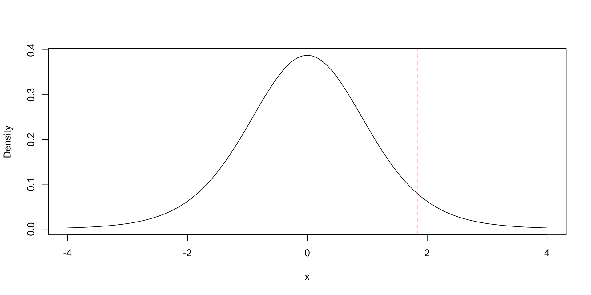
Task 2

Try this

What would change if the alternative hypothesis were "less" instead of "greater"?

sales <- c(11.2, 10.3, 12.0, 9.8, 11.5, 10.7, 12.2, 11.9, 10.9, 10.5)
xbar <- mean(sales)
s <- sd(sales)
n <- length(sales)

# Perform your work below this line

Discuss

Why do we use only one tail of the t-distribution here? How does it relate to directional hypotheses in economics?

Example 3: Simulating Type I Error

Goal: Verify that under $H_0$, a 5% test rejects about 5% of the time.

set.seed(42)
n <- 20; mu0 <- 0; sd <- 1
sim_results <- replicate(10000, {
  x <- rnorm(n, mu0, sd)
  t_stat <- (mean(x) - mu0) / (sd(x) / sqrt(n))
  abs(t_stat) > qt(0.975, df = n - 1)
})
mean(sim_results)

[1] 0.0493

Task 3

Try this

Repeat for n = 5, n = 30, and n = 100. Does the rejection proportion stay near 0.05? Why?

Reflect

How does sample size influence the variability of the t-statistic? What does this say about small-sample inference?

Example 4: Asymptotic z-test

set.seed(1)
x <- rlnorm(2000, meanlog = 0, sdlog = 1)
mu0 <- exp(0.5)
z_stat <- (mean(x) - mu0) / (sd(x)/sqrt(length(x)))
p_val <- 2 * (1 - pnorm(abs(z_stat)))
c(z_stat, p_val)

[1] 0.7404698 0.4590150

# Compare with t-test
t.test(x, mu = mu0)


    One Sample t-test

data:  x
t = 0.74047, df = 1999, p-value = 0.4591
alternative hypothesis: true mean is not equal to 1.648721
95 percent confidence interval:
 1.583284 1.793548
sample estimates:
mean of x 
 1.688416

Task 4

Try this

Try again with only 20 observations. Does the z-test still give a reliable result?

Discuss

Why does the Central Limit Theorem justify z-tests for large samples, even when the data are not normal?

Example 5: Two-Sample Difference in Means

Scenario: Suppose we want to know whether two stores in different cities have the same average daily sales.

set.seed(123)
store_A <- rnorm(25, mean = 520, sd = 50)
store_B <- rnorm(25, mean = 550, sd = 55)

Manual two-sample t-test

# Manual two-sample t-test (assuming unequal variances)
mean_A <- mean(store_A); mean_B <- mean(store_B)
sA <- sd(store_A); sB <- sd(store_B)
nA <- length(store_A); nB <- length(store_B)

se_diff <- sqrt(sA^2/nA + sB^2/nB)
t_stat <- (mean_A - mean_B) / se_diff
df <- (se_diff^4) / (((sA^2/nA)^2 / (nA-1)) + ((sB^2/nB)^2 / (nB-1)))
p_val <- 2 * (1 - pt(abs(t_stat), df = df))
c(t_stat, df, p_val)

[1] -2.692191151 47.795889615  0.009756215

Built-in two-sample t-test

# Compare to built-in
t.test(store_A, store_B, var.equal = FALSE)


    Welch Two Sample t-test

data:  store_A and store_B
t = -2.6922, df = 47.796, p-value = 0.009756
alternative hypothesis: true difference in means is not equal to 0
95 percent confidence interval:
 -65.132363  -9.435781
sample estimates:
mean of x mean of y 
 518.3335  555.6176

Task 5

Try this

Change the sample size to 10 for each store and rerun. What happens to the standard error and p-value?

Reflect

Why might smaller samples lead to more uncertainty about the difference in means? How would equal-variance assumption affect results?

Theory: Equal-Variance Two-Sample t-test

In Example 4, we used the Welch’s t-test, which does not assume equal variances. If we instead assume $\sigma_X^2 = \sigma_Y^2,$ we can use the pooled-variance t-statistic, often written as:

\[ U = \frac{\sqrt{m+n-2}(\bar{X}-\bar{Y})}{\sqrt{\frac{1}{m} + \frac{1}{n}}\,\sqrt{s_X^2+s_Y^2}}. \]

Equal-Variance Two-Sample t-test

m <- length(store_A); n <- length(store_B)
sX <- sd(store_A); sY <- sd(store_B)
xbar <- mean(store_A); ybar <- mean(store_B)

# Pooled (equal variance) test
U <- sqrt(m + n - 2) * (xbar - ybar) /
(sqrt(1/m + 1/n) * sqrt(sX^2 + sY^2))
p_val_U <- 2 * (1 - pt(abs(U), df = m + n - 2))
# Welch's version
Welch_t <- (xbar - ybar) / sqrt(sX^2/m + sY^2/n)
df_welch <- (sX^2/m + sY^2/n)^2 /
((sX^2/m)^2/(m-1) + (sY^2/n)^2/(n-1))
p_val_welch <- 2 * (1 - pt(abs(Welch_t), df = df_welch))

data.frame(U_pooled = U, p_val_pooled = p_val_U,
Welch_t = Welch_t, p_val_welch = p_val_welch)

   U_pooled p_val_pooled   Welch_t p_val_welch
1 -13.18899            0 -2.692191 0.009756215

Reflect

When is the pooled version appropriate? How do results compare with the unequal-variance test when sample sizes or variances differ?

Example 6: Testing Correlation

Goal: Test whether there is a significant correlation between two variables X and Y. We’ll test the null hypothesis $H_0: \rho = 0$ against the alternative $H_1: \rho \neq 0$.

First, simulate the data

set.seed(100) 
n=50000
X <- rnorm(n, mean = 10, sd = 3)
Y <- 5 + 0.8 * X + rnorm(n, mean = 0, sd = 2)

Using asymptotic z-test

# sample correlation
r <- cor(X, Y)
# Asymptotic variance using sample analog (plug-in)
se_hat  <- sqrt((1 - r^2)^2 / n)
# z-statistic and two-sided p-value
z_stat <- (r - 0) / se_hat
p_val  <- 2 * (1 - pnorm(abs(z_stat)))
ci_lower <- r - qnorm(0.975)*se_hat
ci_upper <- r + qnorm(0.975)*se_hat

# Display results
cat(paste("Asymptotic z-test for correlation\n","-----------------------------------\n",
sprintf("r = %.4f", r),sprintf(", SE = %.4f\n", se_hat),sprintf("z-statistic = %.3f, ", z_stat),
sprintf("p-value = %.4g\n", p_val),sprintf("CI = (%.4g , %.4g)", ci_lower,ci_upper)))

Asymptotic z-test for correlation
 -----------------------------------
 r = 0.7685 , SE = 0.0018
 z-statistic = 419.660,  p-value = 0
 CI = (0.7649 , 0.7721)

Compare to t-test based correlation test

# Compare to cor.test()
cat("Built-in cor.test() results (t-based)\n")

Built-in cor.test() results (t-based)

print(cor.test(X, Y))


    Pearson's product-moment correlation

data:  X and Y
t = 268.53, df = 49998, p-value < 2.2e-16
alternative hypothesis: true correlation is not equal to 0
95 percent confidence interval:
 0.7648525 0.7720309
sample estimates:
      cor 
0.7684658

Task 6

Try this

Generate new samples with weaker correlation (e.g., use Y <- 5 + 0.2 * X + rnorm(n, 0, 2)). Does the correlation remain significant? How big $n$ should be so that the t-based and normal-based test converge?

Reflect

How does the correlation test relate to slope significance in simple linear regression?

Challenge Problem: Sleep Hours

Question: Do college students sleep less than 7 hours per night?

set.seed(10)
sleep_hours <- rnorm(40, mean = 6.7, sd = 1)
# H0: mu = 7 vs H1: mu < 7
t_stat <- (mean(sleep_hours) - 7) / (sd(sleep_hours) / sqrt(40))
p_val <- pt(t_stat, df = 39)
c(t_stat, p_val)

[1] -5.032903e+00  5.644199e-06

# Compare to built-in
t.test(sleep_hours, mu = 7, alternative = "less")


    One Sample t-test

data:  sleep_hours
t = -5.0329, df = 39, p-value = 5.644e-06
alternative hypothesis: true mean is less than 7
95 percent confidence interval:
     -Inf 6.529234
sample estimates:
mean of x 
 6.292324

Challenge Task

Follow-up

Repeat with n = 100.
Compare manual and R results.
Interpret the result in context.

Think

If this were a real study, what confounding factors might affect your inference about student sleep?

Wrap-Up

✅ Key Takeaways

Always state $H_0$, $H_1$, $\alpha$, and the test direction clearly.
Manual calculation reinforces understanding; R simplifies application and avoids arithmetic mistakes.
For large $n$, t-tests approximate z-tests (asymptotic normality).
Choice between pooled and Welch t-test depends on whether variances are assumed equal.
Correlation tests can be done using either t-based or z-based asymptotic methods.

Wrap-Up

Test Type	Statistic	Built-in Function	Manual Formula
Two-sided hypothesis	t-stat	`t.test(x, mu=c)`	$(\bar{x} - c) / (s_x / \sqrt{n})$
One-sided hypothesis	t-stat	`t.test(..., alternative="greater")`	Use one tail of t-distribution
Asymptotic (general)	z-stat	manual	$(\hat{\theta}-\theta_0)/se(\hat{\theta})$
Two-sample mean (Welch)	t-stat	`t.test(x, y, var.equal=FALSE)`	$(\bar{x}_1 - \bar{x}_2)/\sqrt{s_1^2/n_1 + s_2^2/n_2}$
Two-sample mean (Pooled)	t-stat	`t.test(x, y, var.equal=TRUE)`	$\sqrt{m+n-2}\dfrac{\bar{x}-\bar{y}}{\sqrt{1/m+1/n}\sqrt{s_x^2+s_y^2}}$
Correlation	z-stat	`cor.test()`	$(r - \rho_0)/\sqrt{(1-r^2)^2/n}$

Submission

Replicating and submitting pdf worth 70 points, each Task (Try and Reflect/Discuss) worth 5 points, Challenge Problem worth extra 5 points.
Change the name in the first page to your group member
Submit the rendered PDF by group on Canvas assignment by Monday 11:59 (Focus on presentation this week)

Note

If you want to try different examples, modify sample sizes or change the null hypothesis. Record your findings in a markdown cell for submission.

Lab 4: Hypothesis Testing

Plan

Best Costume: Louvre Robbers #1 (Charlotte)

Overview

Submission

Warm-up & Review

Warm-up & Review

Exercise 1: Two-sided t-test

Manual two-sided t-test

Built-in function two-sided t-test

Task 1

Exercise 2: One-Sided t-test

Manual one-sided t-test

Built-in one-sided t-test

Visualize rejection region

Task 2

Example 3: Simulating Type I Error

Task 3

Example 4: Asymptotic z-test

Task 4

Example 5: Two-Sample Difference in Means

Manual two-sample t-test

Built-in two-sample t-test

Task 5

Theory: Equal-Variance Two-Sample t-test

Equal-Variance Two-Sample t-test

Example 6: Testing Correlation

Using asymptotic z-test

Compare to t-test based correlation test

Task 6

Challenge Problem: Sleep Hours

Challenge Task

Wrap-Up

Wrap-Up

Submission

Feedback form